Graph Theory -- Semester-3 -- Mathematics III

#Semester-3

Index

What is a Graph?
Basic Terminology
Types of Graph
Complement of a graph.
Planar Graph
Di-graph (or Directed Graph)
Important Terminologies
Euler Line, Eulerian Circuit and Euler Graph
Hamiltonian path, Hamiltonian Circuit and Hamiltonian Graph
Isomorphic Graphs
Theorems of Graph Theory
Incidence and Adjacency
Matrix Representation of a graph.
Adjacency Matrix
Incidence Matrix
Trees
Spanning Trees
Minimal Spanning Trees
Algorithms for finding the (Minimal Spanning Tree) MST of a Tree.
1. Kruskal's Algorithm
2. Prim's Algorithm

Note : If the equations on the website seem a bit to clumped up/clogged, please go to the resources section and download the PDF. It has better indentation.

What is a Graph?

A graph is a mathematical structure containing 2 sets V and E where V represents a non-empty set of vertices and E represents a non-empty set of edges.

Pasted image 20240610105425.png

Basic Terminology

Trivial Graph : A graph containing only one vertex no edge.
Null Graph: A graph containing n vertices and no edge.
Directed Graph: A graph consisting the direction of edges is called a directed graph.
Undirected Graph: A graph which is not directed.
Self loop in a graph: If edge having the same vertex as both it's end vertices is called a self loop.
Proper edge: An edge which is not self loop is called proper edge.
Multi edge: A collection of two or more vertices having a same end point.

Pasted image 20240610110441.png

Pasted image 20240610110508.png

Types of Graph

Complete Graph: A simple connected graph is said to be complete if each vertex links to every other vertex.
Regular Graph: A graph G is said to be regular if every vertex has the same degree. If the degree of each vertex of graph G is K, then it is called K-regular graph.
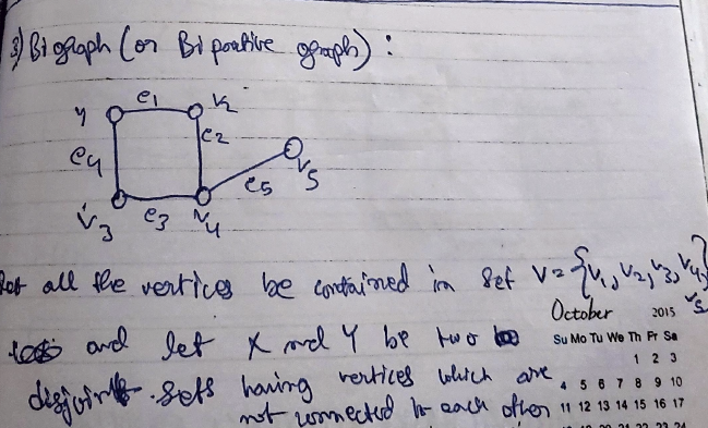
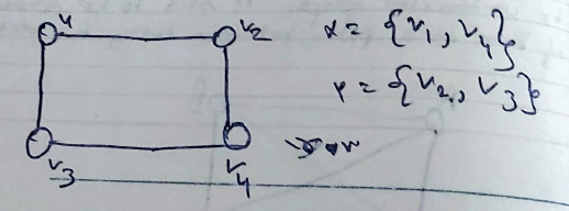
Bi-graph (or Bipartite Graph): Let all the vertices contained in set
$V = {v 1, v 2, v 3, v 4, v 5}$
and let X and Y be two =disjoint sets= having vertices which are not connected to each other :
$X = {v_{1}, v_{4}}$
and
$Y = {v_{3}, v_{2}, v_{5}}$
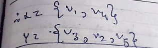
Complete Bi-partite graph: If every vertex in X is disjoint with every vertex in Y, then the graph is called a complete Bi-partite graph.
Subgraph : Let there be a graph G(V, E), V and E being the two sets for it's vertices and edges. Let V' and E' be the subsets of V and E respectively. Thus G(V', E") is a graph and subgraph of G(V, E).

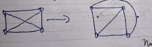
Complement of a graph.

The complement of a graph is basically the :

connection of previously unconnected vertices

and

removal of the connection of currently connected vertices

Pasted image 20240610112123.png

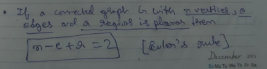
Planar Graph

A graph which can be drawn in a plane so that it's edges do not cross are called planar graphs.

Pasted image 20240610112458.png

Self loops or parallel edges may be allowed here.

Pasted image 20240610124150.png

Pasted image 20240610124215.png

Di-graph (or Directed Graph)

It is a type of graph where each edge has a direction.

Pasted image 20240610113816.png

The starting vertex is called the initial vertex.

The vertex which has no incoming edges but only outgoing edges is called a source.

The vertex which has only incoming edges and no outgoing edges is called a sink.

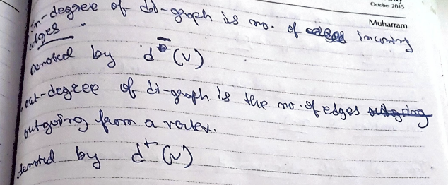
The In-degree of a di-graph is the number of incoming edges.

Denoted by $$ d^-(v) $$
Out- degree of di-graph is the number of edges outgoing from a vertex.

Denoted by $$ d^+(v) $$

Pasted image 20240610114208.png

Important Terminologies

What is a Walk?

A walk is simply the traversal of all vertices in a graph and coming back to the initial vertex.

Pasted image 20240610114408.png

What is a Trail?

A trail is also a walk which traverses all the vertices and ending at the last vertex, where no edges are repeated and the starting vertex is not equal to the ending vertex.

Pasted image 20240610114803.png

What is a Circuit?

A circuit is a closed trail where the starting vertex is the same as the ending vertex, i.e the walk ends at the initial vertex (no edges are repeated).

So, taking the graph above, the Circuit would be

v1 -> v2 -> v3 -> v4 -> v5 -> v6 -> v7 -> v1

as no edges are repeated (only accessed once).

What is a Path?

A path is a walk where neither edges nor vertices are repeated and the start vertex is not equal to the end vertex, i.e the walk ends at the last vertex of the graph.

In the graph above, the sequence,

v1 -> v2 -> v3 -> v4 -> v5 -> v6 -> v7

is applicable as a path as no edges or vertices are repeated.

What is a Cycle?

A cycle is a =closed Path= where the =starting vertex is the same as the ending vertex= , i.e =the walk ends at the initial vertex of the graph=.

In the graph above, the sequence:

v1 -> v2 -> v3 -> v4 -> v5 -> v6 -> v7 -> v1

is applicable as a cycle since no intermediate edges or vertices except the starting vertex are repeated and the traversal ends at the starting vertex of the graph.

Euler Line, Eulerian Circuit and Euler Graph

What is a Euler line?

A Euler line is a trail where each edge is visited exactly once.

What is a Eulerian Circuit?

A circuit that contains all the edges(without repeating any) is called a Eulerian circuit.

What is a Euler graph?

A graph that contains a Eulerian circuit is called a Euler Graph.

Pasted image 20240610115611.png

Hamiltonian path, Hamiltonian Circuit and Hamiltonian Graph

What is a Hamiltonian path?

A path which obtains every vertex of a graph exactly once is called a Hamiltonian Path.

What is a Hamiltonian circuit?

A circuit which passes through every vertex at least once is called a Hamiltonian circuit (ends at the starting vertex).

What is a Hamiltonian graph?

A graph which contain a Hamiltonian circuit is called a Hamiltonian graph.

Pasted image 20240610120109.png

Note : A Hamiltonian circuit will always have a Hamiltonian path but the reverse is not always true.

Pasted image 20240610120318.png

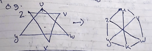
Isomorphic Graphs

Two graphs G and G' are said to be isomorphic if

They have the same number of edges.
They have the same number of vertices.
The vertices in graph G' should have the same degree as the vertices in the graph G.

Pasted image 20240610120516.png

Vertex-disjoint and Edge disjoint Graphs

Two graphs called vertex disjoint if they have no vertex in common .

Two graphs are called edge disjoint if they have no edge in common .

Pasted image 20240610112737.png

Theorems of Graph Theory

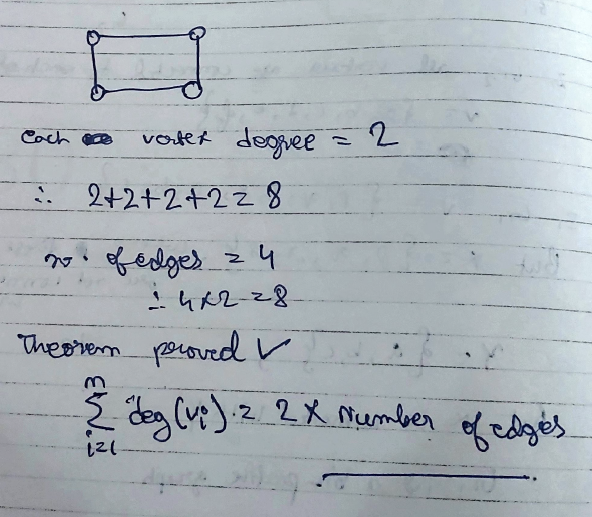
1. Handshaking Theorem/ The first theorem of graph theory.

This theorem states that the "sum of the degree of the vertices of a graph is equal to twice the number of edges in a graph G".

Pasted image 20240610113207.png

2. The degree of any vertex in a simple graph with any vertices is n-1.

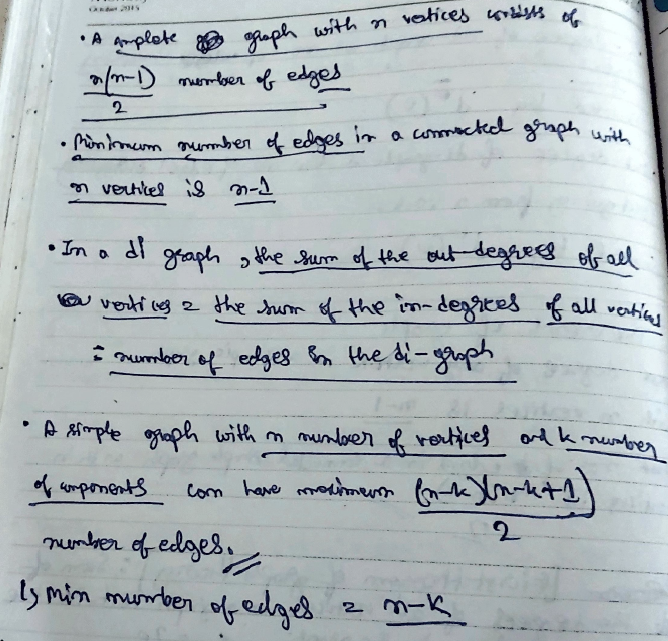
3. ==The maximum number of edges in a connected simple graph with n vertices is :

n(n-1)/2==.

4. The number of odd vertices in any graph is even.

5. Minimum number of edges in a connected graph with n vertices in n-1.

Pasted image 20240610120623.png

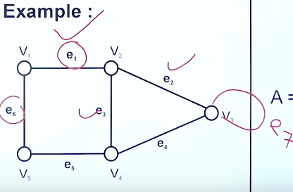
Incidence and Adjacency

flowchart LR;
	v1--e1-->v2

Let there be an edge $e_{1}$ joining two vertices $v_{1}$ and $v_{2}$

Therefore one can say that edge $e_{1}$ is incident for $v_{1}$ and $v_{2}$

And the vertices $v_{1}$ and $v_{2}$ are adjacent on edge $e_{1}$ .

Edge, incident for vertices. Vertices adjacent on edge.

Matrix Representation of a graph.

https://www.youtube.com/watch?v=17erhldpZ8E&list=PLU6SqdYcYsfLV24T0XVb3z3mjl8QG0EBN&index=3

Adjacency Matrix

Adjacency matrix: Let $a_{i j}$ denote the number of edges connecting vertices ( $v_{i}$ , $v_{j}$ ), then A = $[a_{i j}]_{m X m}$ is called an adjacency matrix of a graph G, if $a_{i j}$ = 1 if the vertices $v_{1}$ and $v_{2}$ are connected, and 0 if they are not connected.

Let's understand this using an example.

Pasted image 20241105214553.png

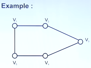
Vertex	$v_{1}$	$v_{2}$	$v_{3}$	$v_{4}$	$v_{5}$
$v_{1}$
$v_{2}$
$v_{3}$
$v_{4}$
$v_{5}$

So this is how we setup our adjacency matrix.

Now we see that $v_{1}$ is connected to $v_{2}$ and $v_{5}$ .

So we will fill the values with 1 under them and the rest with 0.

Vertex	$v_{1}$	$v_{2}$	$v_{3}$	$v_{4}$	$v_{5}$
$v_{1}$	0	1	0	0	1
$v_{2}$
$v_{3}$
$v_{4}$
$v_{5}$

Now we see $v_{2}$ is connected both to $v_{1}$ and $v_{3}$ . So we fill their places with 1.

Vertex	$v_{1}$	$v_{2}$	$v_{3}$	$v_{4}$	$v_{5}$
$v_{1}$	0	1	0	0	1
$v_{2}$	1	0	1	0	0
$v_{3}$
$v_{4}$
$v_{5}$

For $v_{3}$ , it's connected to $v_{2}$ and $v_{4}$ , so we fill 1 under their places.

Vertex	$v_{1}$	$v_{2}$	$v_{3}$	$v_{4}$	$v_{5}$
$v_{1}$	0	1	0	0	1
$v_{2}$	1	0	1	0	0
$v_{3}$	0	1	0	1	0
$v_{4}$
$v_{5}$

For $v_{4}$ , it's connected to $v_{3}$ and $v_{5}$ . So we fill 1 under their places.

Vertex	$v_{1}$	$v_{2}$	$v_{3}$	$v_{4}$	$v_{5}$
$v_{1}$	0	1	0	0	1
$v_{2}$	1	0	1	0	0
$v_{3}$	0	1	0	1	0
$v_{4}$	0	0	1	0	1
$v_{5}$

For $v_{5}$ , it's connected to $v_{4}$ and $v_{1}$ . So we fill 1 under their places.

Vertex	$v_{1}$	$v_{2}$	$v_{3}$	$v_{4}$	$v_{5}$
$v_{1}$	0	1	0	0	1
$v_{2}$	1	0	1	0	0
$v_{3}$	0	1	0	1	0
$v_{4}$	0	0	1	0	1
$v_{5}$	1	0	0	1	0

So this is our final adjacency matrix.

Example 2: Self loops and Parallel Edges in Adjacency Matrix

Let's say that this diagram was now modified to look like this :

Pasted image 20241105215658.png

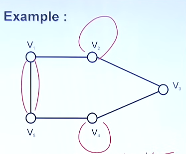
So here, self-loops would count as 1, towards the same vertex, and the extra paths would add up as well.

So the modified adjacency matrix would be:

Vertex	$v_{1}$	$v_{2}$	$v_{3}$	$v_{4}$	$v_{5}$
$v_{1}$	0	1	0	0	3
$v_{2}$	1	1	1	0	0
$v_{3}$	0	1	0	1	0
$v_{4}$	0	0	1	1	1
$v_{5}$	3	0	0	1	0

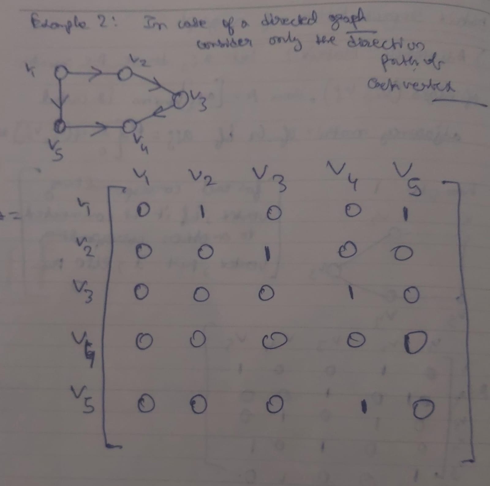
Since there are 3 edges from $v_{1}$ to $v_{5}$ and vice-versa, and self loops in vertices $v_{2}$ and $v_{4}$ .

Example 3 : Adjacency matrix for Directed Graphs

In case of a directed graph, where the edges follow a certain direction only, we need to consider only the direction in which the edge is flowing, not the reverse.

Incidence Matrix

Let G be a graph with m vertices $V_{1}$ , $V_{2}$ , $V_{3}$ and n edges, $e_{1}$ , $e_{2}$ , $e_{3}$ , ..... , $e_{n}$ .

Let a matrix M = $[m_{i j}]_{m X n}$ , $m_{i j}$ = 1, if the vertex is incident on the edge.

$m_{i j}$ = 0, if the vertex is not incident on the edge.

$m_{i j}$ = 2, if the vertex is at the end of a self loop.

Let's take an example to understand this :

Pasted image 20241106091723.png

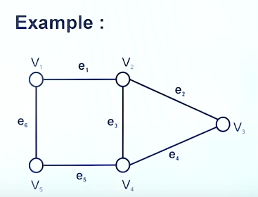
So this is our initial incidence matrix.

Vertex	$e_{1}$	$e_{2}$	$e_{3}$	$e_{4}$	$e_{5}$	$e_{6}$
$v_{1}$
$v_{2}$
$v_{3}$
$v_{4}$
$v_{5}$

So we see vertices $v_{1}$ and $v_{2}$ are incident on edge $e_{1}$
And vertices $v_{1}$ and $v_{5}$ are incident on edge $e_{6}$ .

Therefore we fill 1 under their places for the respective vertices, and the rest with 0.

Vertex	$e_{1}$	$e_{2}$	$e_{3}$	$e_{4}$	$e_{5}$	$e_{6}$
$v_{1}$	1	0	0	0	0	1
$v_{2}$	1
$v_{3}$
$v_{4}$
$v_{5}$						1

Now we see vertices $v_{2}$ and $v_{3}$ are incident on edge $e_{2}$ .
And vertices $v_{2}$ and $v_{4}$ are incident on edge $e_{3}$ .

Therefore we fill 1 under their places for the respective vertices, and the rest with 0.

Vertex	$e_{1}$	$e_{2}$	$e_{3}$	$e_{4}$	$e_{5}$	$e_{6}$
$v_{1}$	1	0	0	0	0	1
$v_{2}$	1	1	1	0	0	0
$v_{3}$		1
$v_{4}$			1
$v_{5}$						1

Now we see vertices $v_{3}$ and $v_{4}$ are incident on edge $e_{4}$ .

And vertices $v_{4}$ and $v_{5}$ are incident on edge $e_{5}$ .

Therefore we fill 1 under their places for the respective vertices, and the rest with 0.

Vertex	$e_{1}$	$e_{2}$	$e_{3}$	$e_{4}$	$e_{5}$	$e_{6}$
$v_{1}$	1	0	0	0	0	1
$v_{2}$	1	1	1	0	0	0
$v_{3}$	0	1	0	1	0	0
$v_{4}$	0	0	1	1	1	0
$v_{5}$	0	0	0	0	1	1

And this is our resultant incidence matrix.

Now let's say the graph was modified to have a new edge $e_{7}$ , on a self loop.

Pasted image 20241106093351.png

We see the vertex $v_{3}$ is incident on the edge $e_{7}$ which is bound in a self loop.

So self loops in incidence matrix are counted as 2.

Vertex	$e_{1}$	$e_{2}$	$e_{3}$	$e_{4}$	$e_{5}$	$e_{6}$	$e_{7}$
$v_{1}$	1	0	0	0	0	1	0
$v_{2}$	1	1	1	0	0	0	0
$v_{3}$	0	1	0	1	0	0	2
$v_{4}$	0	0	1	1	1	0	0
$v_{5}$	0	0	0	0	1	1	0

And this would be the resultant incidence matrix.

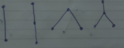
Trees

A tree is a connected graph without any loops or circuits.

Example :

Pasted image 20240610131118.png

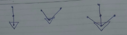
Rooted Tree

A rooted tree is a tree in which vertex acts as the root(initial vertex) of the tree.

Pasted image 20240610131211.png

Binary Tree

A binary tree is defined as a tree in which there is exactly one vertex of degree two which acts as the root vertex and the remaining vertices could be of degrees one or three but not two.

Pasted image 20240610131427.png

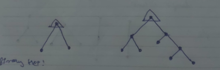
These are binary trees.

However:

Pasted image 20240610131444.png

This is not a binary tree as there is one vertex other than the root which has a degree of 2.

The vertices at the end of the tree (or leaf nodes) are called pendant vertices since they have a degree of 1.

Pasted image 20240610131549.png

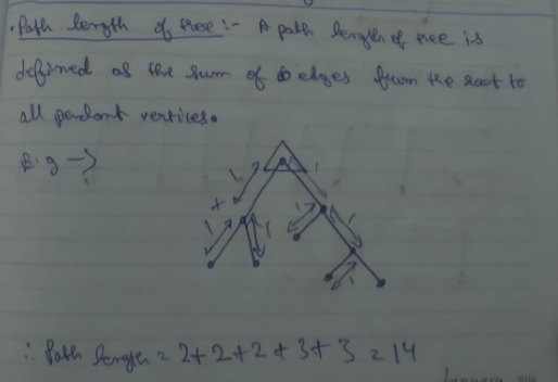
Path length of a tree

A path length of a tree is defined as the sum of edges from the root to all the pendant vertices.

Pasted image 20240610131827.png

Spanning Trees

Video explanation (Recommended to watch) :

https://www.youtube.com/watch?v=f30rxGvPWPo&list=PLU6SqdYcYsfLV24T0XVb3z3mjl8QG0EBN&index=9

A spanning tree is basically a subgraph of a graph G.

Pasted image 20240610131958.png

ST = Spanning Trees

Some examples on Spanning Trees

Pasted image 20240610132053.png

Pasted image 20240610132128.png

Pasted image 20240610132155.png

Pasted image 20240610132207.png

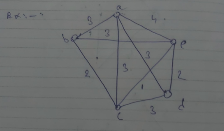
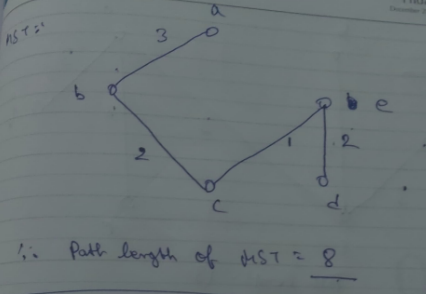
Minimal Spanning Trees

Let G be a weighted graph. A minimal spanning tree of G is a spanning tree of minimum weight.

Pasted image 20240610132420.png

Graph G.

Pasted image 20240610132431.png

Pasted image 20240610132443.png

However the MST of G will be the spanning tree whose combined length is the least of all the spanning trees.

Pasted image 20240610132527.png

Algorithms for finding the (Minimal Spanning Tree) MST of a Tree.

https://www.youtube.com/watch?v=f30rxGvPWPo&list=PLU6SqdYcYsfLV24T0XVb3z3mjl8QG0EBN&index=9 (MST, Kruskal's and Prim's algorithms)

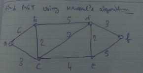
1. Kruskal's Algorithm

Step 1. Choose an edge of minimal weight.
Step 2. At each step, choose the edge whose inclusion will not create a circuit.
Step 3. If a graph G has n vertices then stop after (n-1) edges.

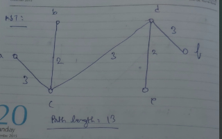
Example of Kruskal's algorithm:

Pasted image 20240610132751.png