https://www.youtube.com/playlist?list=PLF-vWhgiaXWM7Iri0t_AjBfv51tF28PEy (Full playlist link)

Index

Class 12 level recap

1. Integral Calculus Recap
2. Basic Integral Formulae
3. Some basic trigonometric identities
4. Methods of integration
5. 1. U-substitution
6. 2. Integration by Parts -- The easy method.
7. 3. Integration by partial fractions -- An easy method

College Stuff (Calculus -3)

8. Double Integrals
9. Changing of order of integration
10. What is changing of order of integration?
11. When can you NOT change the order of integration.
12. Triple Integrals
13. Change of variables (Cartesian to Polar)
14. When to change from cartesian to polar variables?
15. The Jacobian determinant.
16. How to calculate the determinant of a 2x2 matrix?
17. How to calculate the determinant of a 3x3 matrix?
18. Back to conversion of Cartesian to Polar co-ordinates
19. Green's Theorem (Statement only) (and detailed examples included)
20. Gauss's Theorem (Statement only) (and detailed examples included)
21. Stokes's Theorem (Statement only) (and detailed examples included)

Note : If the equations on the website seem a bit to clumped up/clogged, please go to the resources section and download the PDF. It has better indentation.

Integral Calculus Recap

A problem well defined, is a problem half solved -- Charles Kettering

https://www.youtube.com/watch?v=hXOrQ0Ao4UE&list=PLF-vWhgiaXWM7Iri0t_AjBfv51tF28PEy&index=1&pp=gAQBiAQB

The above link points to a full comprehensive recap of class 12 recap. Watch it only if you have time.

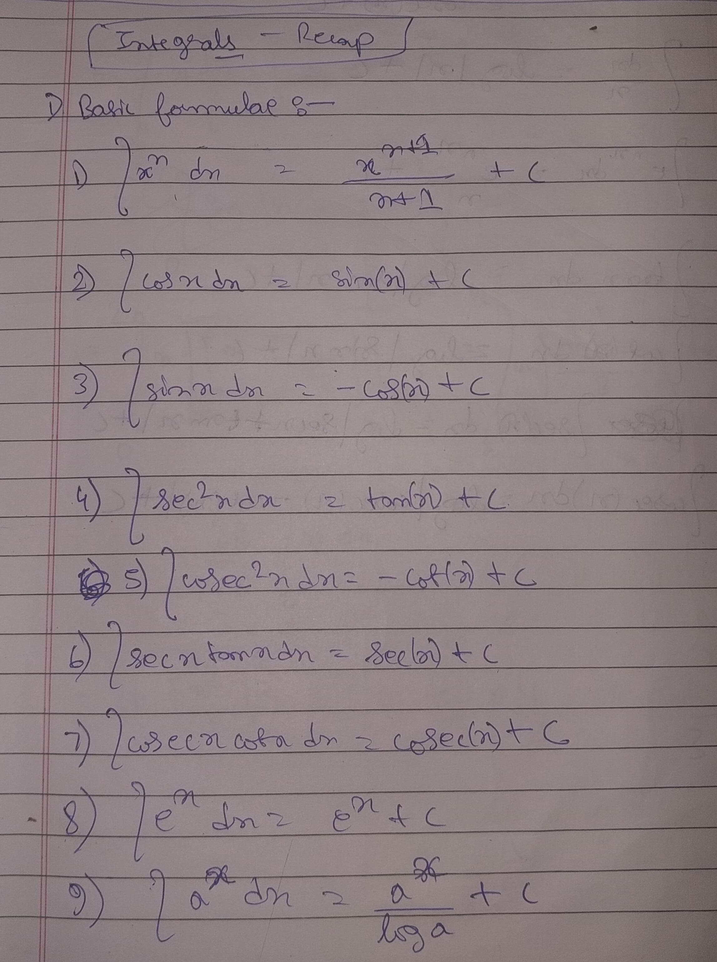
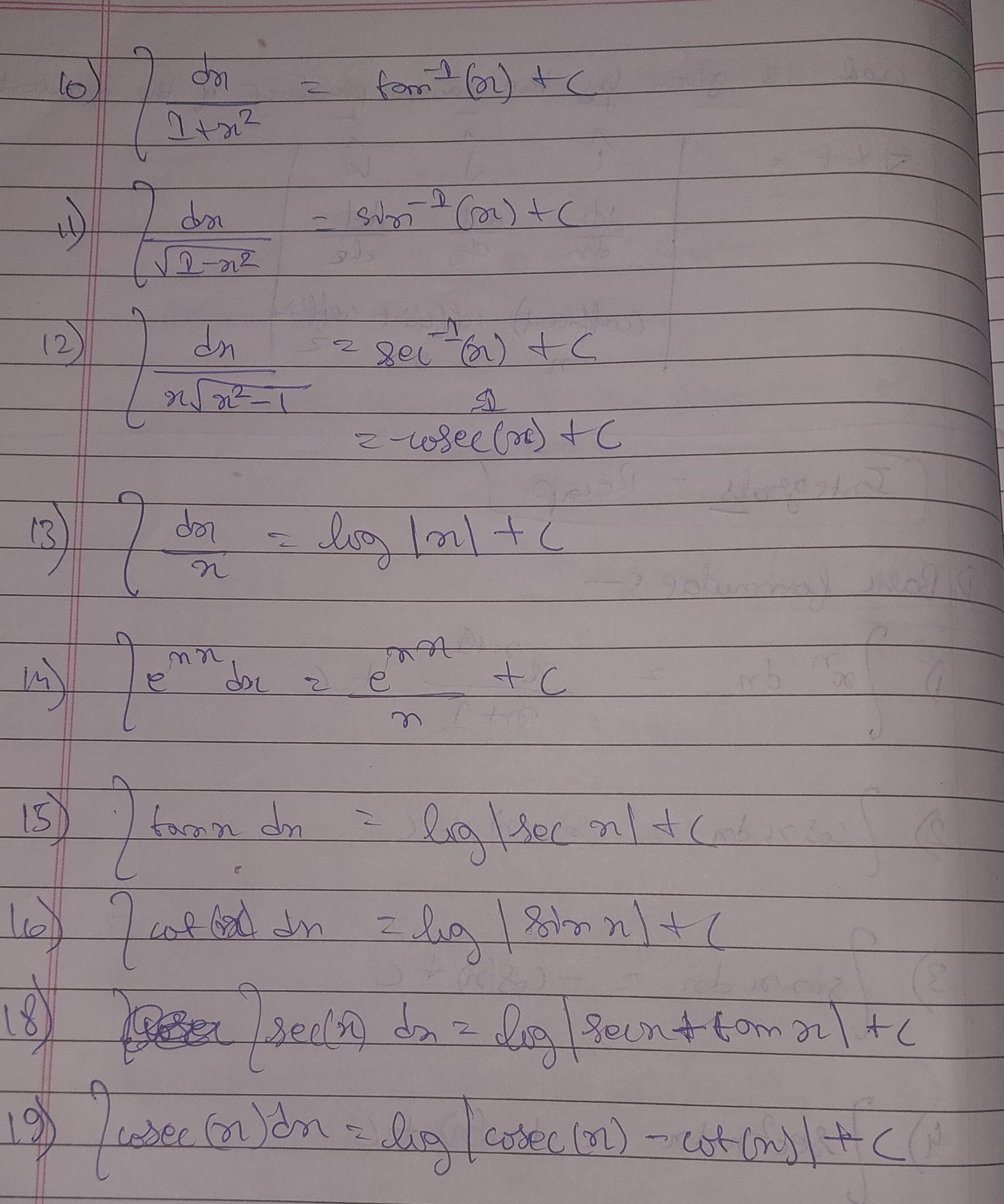
Basic Integral Formulae

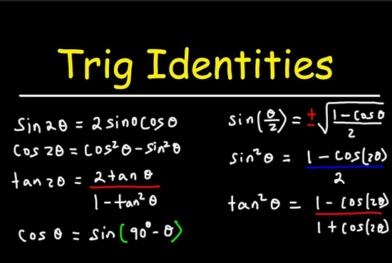
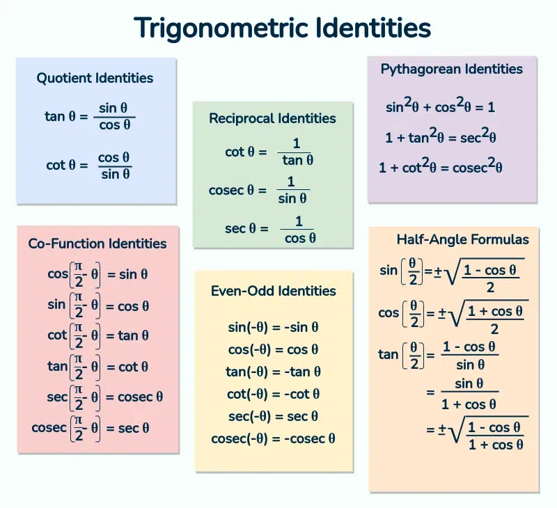
Some basic trigonometric identities

https://www.youtube.com/watch?app=desktop&v=m1OitPmkydY

https://www.geeksforgeeks.org/trigonometric-identities/

https://www.geeksforgeeks.org/trigonometry-table/

Methods of integration

1. U-substitution

So let's say we have an integral

To solve this using u-substitution, we need to:

1. set $x=g(t)$.
2. Differentiate both sides
3. So, we get : $${dx} = g'(t).dt$$
   And then we replace the value of $x$ and $dx$ in the original equation to get:

Example 1 :

1. $$\int sin(mx)dx$$

Let us set $mx=t$ and differentiate both sides w.r.t $x$, we get :

And thus we replace $dx$ in the original equation to get:

or , $$\frac{-cos(mx)}{m} + C$$

Example 2

Let $$1+x^2 = t$$

or $$\implies 0 + 2x = \frac{dt}{dx}$$
or, $$2x dx = dt$$
Replacing this in the original equation,

or ,

2. Integration by Parts -- The easy method.

https://www.youtube.com/watch?v=2I-_SV8cwsw&list=PLF-vWhgiaXWM7Iri0t_AjBfv51tF28PEy&index=2

This is called the D-I method. Differentiate-Integrate. (also known as the LIATE method)

Example 1.

So let's say we have this integral here :

We need to make a small table.

The D column represents differentiation and I column represents integration.

Now we choose each term to be either differentiated or integrated.

Here the easy choice seems to differentiate $x^2$ and integrate $sin(3x)$

Now we continue the respective operations on both sides for a while.

Each column having alternating signs.

What to differentiate and what to integrate?

• Inverse trigonometric functions (like $ta{n}^{-1}$, $si{n}^{-1}$) — differentiate these if present.
• Logarithmic functions (like ln(x)) — differentiate these if present.
• Algebraic functions (like $x^2$, $x$, constants) — differentiate these if no inverse or logarithmic terms are present.
• Trigonometric functions (like $sin(x)$, $cos(x)$) — differentiate these if there are no inverse, logarithmic, or algebraic terms to use.
• Exponential functions (like $e^x$, $a^x$) — these are typically integrated as a last choice.

When to stop the operations:

1. If the column of D reaches 0.
2. If the products of a row (product of both the value of D and I) can be integrated.
3. If any the products of any row (product of both the value of D and I) result in the original integral.

So here we see that the column of D has reached 0.

So we multiply downwards, diagonally, along with each respective sign, and write them together for the final answer.

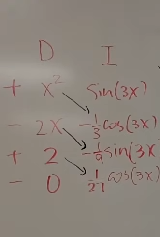
Like this.

So the final answer becomes,

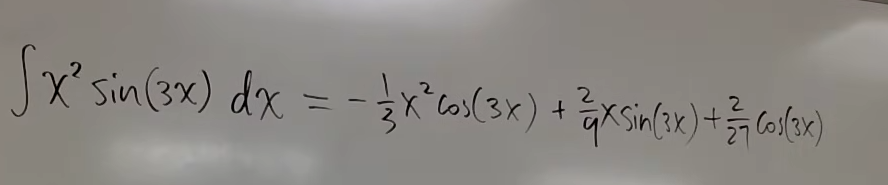
Example 2

Let's say we have another integral

Example 3:

Let's say we have another integral, $$e^x.sin(x)dx$$

Remembering our rules, we differentiate $e^x$, since functions like $e^x$ are integrated as a last choice. And the remaining $sin(x)$ will be differentiated.

So ,

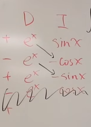
So we stop the operations and write diagonal products first.

or $$2\int{e^x.sin(x)dx} = e^{x}.[sin(x)-cos(x)]$$
or, $$\int{e^x.sin(x)dx} = \boxed{\frac{e^{x}.[sin(x)-cos(x)]}{2}}$$

3. Integration by partial fractions -- An easy method

https://www.youtube.com/watch?v=OFEfGtCsVKg&list=PLF-vWhgiaXWM7Iri0t_AjBfv51tF28PEy&index=4&pp=gAQBiAQB

This method can only be applied if the denominator can be factorized into linear factors

or that in denominator power of $x$ is 1, or it is a product of terms in which power of $x$ is 1.

Example 1

So let's say we have an integral :

We can see that it's denominator is in the form of a product of linear factors.

So the way to tackle this, is to take one term at a time.

We first select $(x-1)$.

Equate this term to 0. We get $x=1$.

Now we apply this value back in the original equation, but there's a twist.

We modify this part of the process by removing the selected term from denominator, but instead placing it in the form of a natural log (log or $ln$), and we don't substitute the value of $x$ in that log term.

1. So, for $(x-1)$

or $$\frac{-ln(x-1)}{6}$$
2. For $(x+2)$, we get $x=-2$

or $$\frac{2(-2) - 1}{(-2-1)(-2-3)}ln(x+2)$$

or $$\frac{-5.ln(x+2)}{15} = \frac{-ln(x+2)}{3}$$
3. For $(x-3)$, we get $x=3$.

or $$\frac{2(3) - 1}{(3-1)(3+2)}.ln(x-3)$$
or $$\frac{5.ln(x-3)}{10} = \frac{ln(x-3)}{2}$$
Finally we put all the obtained terms together along with their signs.

as our complete answer.

The given video link has another example on this.

Double Integrals

https://www.youtube.com/watch?v=BJ_0FURo9RE&list=PLF-vWhgiaXWM7Iri0t_AjBfv51tF28PEy&index=5

Example 1

Let's say we have an integral here, $$\int_{0}^{2}\int_{1}^{3}{xy^2}dydx$$
In double (or triple integrals), the order of integration matters. Whether you want to integrate in terms of $y$ or $x$ or $z$ (triple integrals) first, that depends on you.

So here we follow which variable is given first. The first variable is $dy$.

So we integrate with respect to $y$ first.

or $$\int_{0}^{2}x. [\frac{3^3}{3} - \frac{1^3}{3}]dx$$
or, $$\int_{0}^{2}\frac{26x}{3}. dx$$
or $$\frac{26}{3}.\int_{0}^{2}xdx$$
or, $$\frac{26}{3}.[\frac{x^2}{2}]{0}^{2}$$
or $$\frac{26}{3}.\frac{4}{2}$$
Thus finally, $$\int^{2}\int_{1}^{3}{xy^2}dydx = \boxed{\frac{52}{3}}$$

Example 2

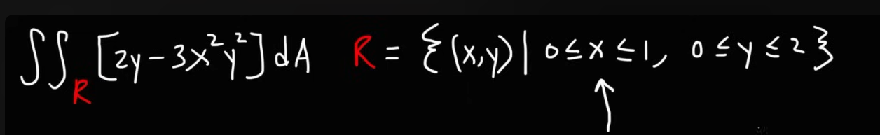
So we have this integral right here,

where $R=\{(x,y)|0\le x\le 1,0\le y\le 2\}$

So we need to find the upper and lower limits of $x$ and $y$.

Following the given set, we see that $x$ lies between $0$ and $1$.

And $y$ lies between $0$ and $2$.

Therefore the integral becomes, $$\int_{0}^{1}\int_{0}^{2}[2y - 3x^2y^2]dxdy$$
While applying the limits we follow the order of the variables in the given set, which in this case, $x$ comes first, followed by $y$

Now it's business as usual. We can solve the integral in the same way we did before.

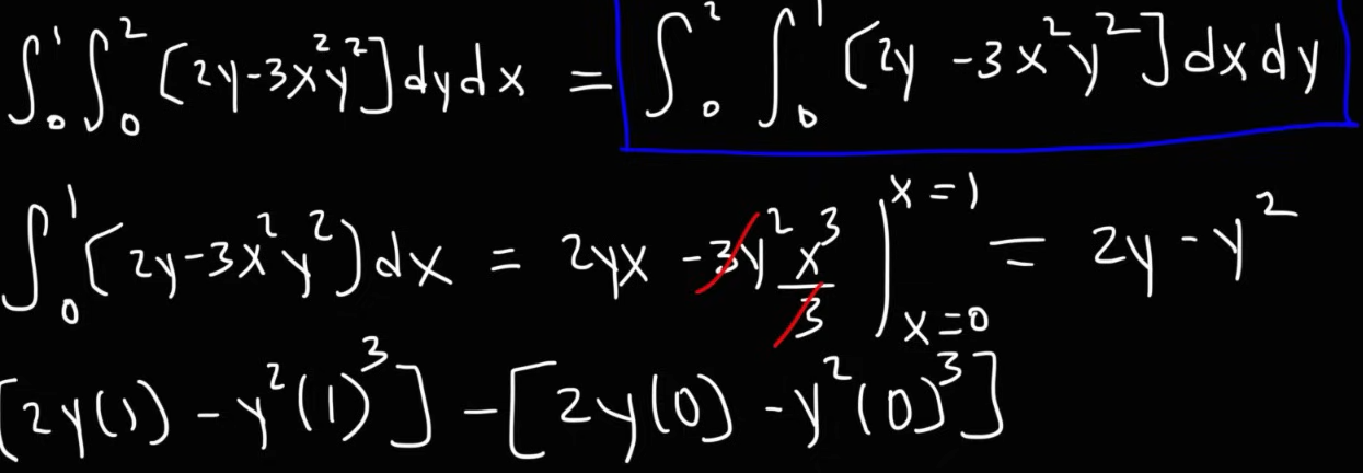
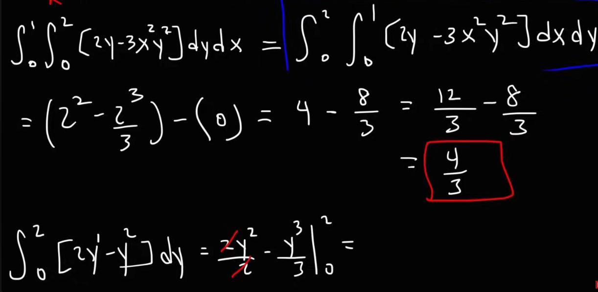
Yeah, I decided to save a bit of time on this one by taking screenshots. Typing and rendering the equations properly is a really time consuming process.

Changing of order of integration

Sometimes we cannot integrate the given question in the given order of variables as it is.

What is changing of order of integration?

Suppose we have an integral,

To change the order of integration, we need to swap both the dx and dy AND their respective limits.

So after changing of order of integration, the new integral would appear as:

Notice that the limits of x and y have swapped respectively when the variables did.

You cannot swap just the variables and keep their limits as they were. This will invalidate the logic of the equation, which will be explained further down the line.

Why do we change the order in integration?

• Sometimes it's easier to evaluate a double integral by changing the order of integration, especially when the region $R$ is more naturally described in one order than another.
• The process involves identifying the new limits of integration for the variables after switching the order.

When can you NOT change the order of integration.

Suppose we have an integral :

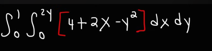
In this question, we see that the limits of $x$ has $y$ entangled in it.

So we if we tried to, let's say write the integral as $$\int_{0}^{2y}\int_{0}^{1}[4+2x - y^2]dydx$$
This won't work here.

Since the limits of $x$ are interdependent on $y$. So we need to evaluate $x$ first , apply the limits which contain $y$. Then integrate in terms of $y$.

A better explanation would be :

In the original equation x relies on the changing value of y, so x is not static.

In this equation, where the order is changed $$\int_{0}^{2y}\int_{0}^{1}[4+2x - y^2]dydx$$
y ranges from 0 to 1 for each fixed x, while x ranges from 0 to 2y.

This completely changes the region over which the integral expands.

So, in these type of integrals we need to solve the interdependent limits first.

or

or

or

or

or

Or if you are indeed keen on changing the order here.

So we have our original equation as:

To change the order of integration, we need to analyze the interdependent limits.

So y's new limits will be from 0 to $\frac{x}{2}$

And thus now y will be dependent on a changing $x$ as it goes from $0$ to $2$. Why $2$ you ask?

Well, you ding-dong, since originally, $x=2y$, $x$ is the double of any value of y.

So it naturally makes sense that when y depends on a changing x, the value of x will be double of whatever $y$'s value is. Originally $x$ ranged from 0 to 1, so now double that, the new range will be $0$ to $2$.

And so the new integral will be :

Now you can go ahead and solve the integral.

To sum it all up.

When changing the order of integration we can shift the limits as well, if they are not inter-dependent on each other.

Otherwise to shift the limits as well, their appropriate new limits need to be calculated to keep the region the integral covers, the same.

Triple Integrals

Welcome to the world of 3-D regions where you often pull out your hair trying to figure out the triple integrals!

Example 1

Here's the referenced video link: https://www.youtube.com/watch?v=7iy83x8bv6o&list=PLF-vWhgiaXWM7Iri0t_AjBfv51tF28PEy&index=6

So we have this scary looking monster right here.

Well don't worry, I got the knight right here to defeat this monster!

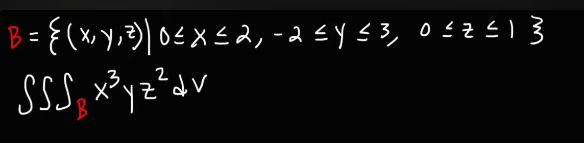
So we have this region of limits B as $\{(x,y,z)|0\le x\le 2,-2\le y\le 3,0\le z\le 1\}$

So this says that the limits of x ranges from 0 to 2.
the limits of $y$ ranges from -2 to 3.
the limits of $z$ ranges from 0 to 1.

So now we can re-write the integral as

As previously stated before, we follow the order of variables when placing the limits in questions like these, from a set.

Now since this is a simple integral with no-interdependent limits, there is no point in changing the order of integration.

We solve the integral as it is.

or $$\int_{0}^{1} \int_{-2}^{3} \frac{yz^2.16}{4}dy,dz$$

or $$4\int_{0}^{1} z^2[\frac{y^2}{2}]_{-2}^{3} dz$$

or $$4\int_{0}^{1} z^2 [\frac{9}{2} - 2]dz$$

or $$4\int_{0}^{1} z^2 \frac{5}{2}dz$$

or $$10[\frac{z^3}{3}]_0^1$$

or $$10 .\frac{1}{3} = \frac{10}{3}$$

Example 2

This time we have a relatively simpler looking question

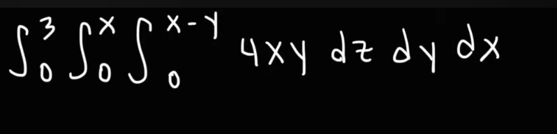
As we see, this integral has interdependent limits. So it's best we solve them in the given specific order to get rid of the dependencies first.

So we start with the integration with respect to $z$.

or

or

or

or

or

or

or

or

or

Change of variables (Cartesian to Polar)

First of all, you might be thinking, what are cartesian and polar variables?

1. Cartesian variables

The cartesian co-ordinate system was introduced by René Descartes , a French (oui baguette) mathematician back in 1637.

This is basically the system where we work with two axes, the x and y axes, with numerical points on them to plot various figures.

Yeah, this.

Normally we represent various diagrams on this plane using variables like x, y, z .... which are known as cartesian variables.

2. Polar variables/Polar co-ordinates

Now the Cartesian system handles 2D objects very nicely, but when dealing with 3D objects, specifically cylinders, spheres, etc, we need a third dimension to work with, which often x, y and z don't make it easy to deal with. Thus, we need the polar coordinate system here. It was developed by Big Daddy Newton (Sir Isaac Newton).

The polar co-ordinate system has variables like r, $\theta$ (pronounced as theta) and sometimes $\varphi$ (pronounced as phi).

Why the name polar?

So yeah most of the type of integrations you can expect on this system are either spheres, or cylinders. At least from Makaut.

When to change from cartesian to polar variables?

1. Symmetry of the Region or Function

If the region of integration or the function itself has circular (radial) symmetry, polar coordinates are often more natural. For example, if you’re integrating over a circular region, like a disk or an annulus, or if the integrand involves terms like $$x^2 + y^2$$, polar coordinates make the setup easier.

In polar coordinates: $$x = rcos\theta$$ and $$y = rsin\theta$$
and $$x^2 + y^2 = r^2$$

2. Simplifying the Integral Expression

When you convert to polar coordinates, the differential element $dx\hspace{0.17em}dy$ , becomes $r\hspace{0.17em}drd\theta$r. This adjustment often simplifies the integrand, especially when it involves $x^2+y^2$ terms. For example:

This $r$ factor can be very helpful in evaluating integrals, especially when combined with radial symmetry, since it often allows you to separate variables or take advantage of simpler limits.

Summary: When to Consider Polar Coordinates

• The region of integration has circular boundaries (disks, rings, etc.).
• The integrand involves terms like $x^2+y^2$
• There is radial symmetry, making polar coordinates a more natural fit.

How to convert from Cartesian to Polar Variables?

https://www.youtube.com/watch?v=a334vcCiZ78&list=PLF-vWhgiaXWM7Iri0t_AjBfv51tF28PEy&index=7

This video tells us how to convert the cartesian variables to polar variables using the Jacobian determinant

So as a pre-requisite we must understand what the Jacobian determinant is.

This part will be re-referenced again in Multi-variable differential calculus.

The Jacobian determinant.

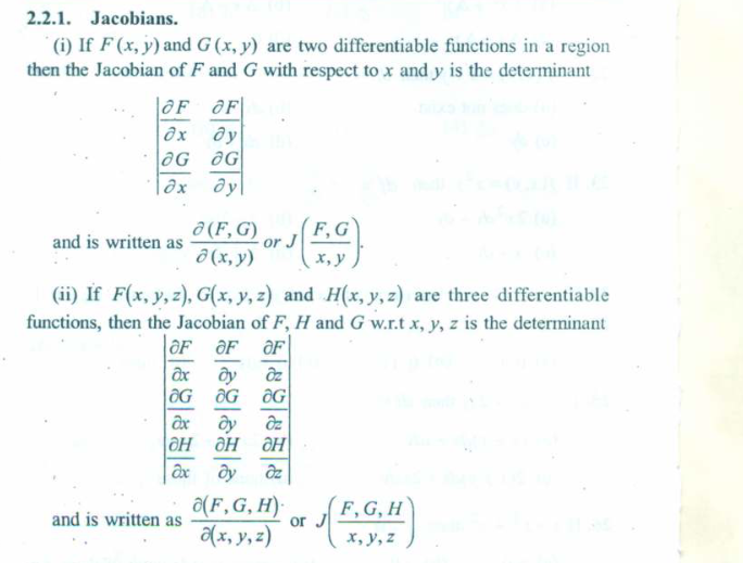
Yeah I saved some time there.

So now, what begs the question is, What is a determinant? What is a Matrix?

Well in-case you are someone who has been out of touch with higher level maths for a long time, I will explain these here.

I will keep this on a strictly need-to-know basis only as we don't want to divert too off track here.

What is a Matrix?

A matrix is a representation are rectangular (2 or 3 or even more) dimensional arrays of real numbers.

For example, this a 3x3 matrix.

And

this is a 2x2 matrix

What is a determinant?

The determinant of a matrix is a single numerical value that is calculated from the elements of a square matrix. It is used to solve systems of linear equations, calculate the inverse of a matrix, and in calculus operations. The determinant is denoted by $|A|$ or $det(A)$.

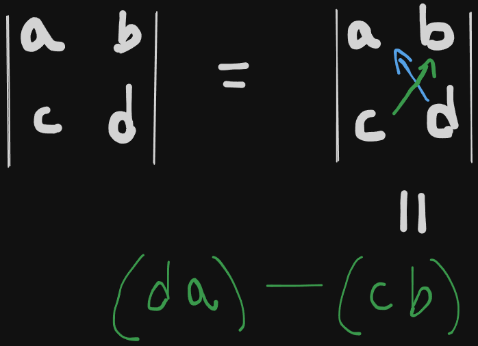
How to calculate the determinant of a 2x2 matrix?

Considering our previous matrix example here :

The determinant of this matrix :

is given by $$[ad] - [bc]$$

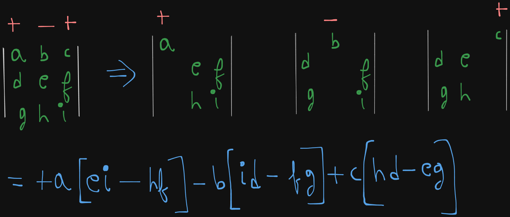
How to calculate the determinant of a 3x3 matrix?

Let's say we have a 3x3 matrix here

The determinant is given by :

which evaluates to :

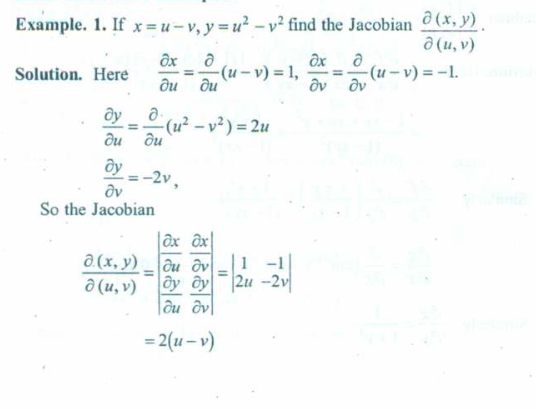
Example 1. Jacobian Determinant

Now that the basic's out of the way, let's practice two examples before we get back to the conversion of cartesian to polar co-ordinates.

Example 2.

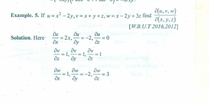
Don't think about the differentiation part too much in here as it's out of context, but will be properly explained in the multi-variable differentiation notes(Assuming you are doing integration first).

Back to conversion of Cartesian to Polar co-ordinates

https://www.youtube.com/watch?v=a334vcCiZ78&list=PLF-vWhgiaXWM7Iri0t_AjBfv51tF28PEy&index=7

(In case you lost the link)

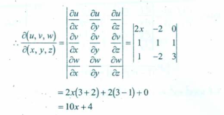
So let's say we have this given integral here: (It's a very important question in general)

We are asked to solve this integral by changing the variables into Polar co-ordinates.

Steps to convert Cartesian to Polar co-ordinates

1. Set $x=rcos\theta$ and $y=rsin\theta$ .

After doing that our integral will look like this :

Yeah, try dressing up a chicken in a duck outfit, that's what the integral is right now.

So we need to :

2. Convert $dydx$ to $drd\theta$ .

Using the Jacobian determinant, we have : $$dx,dy = |J|, dr,d\theta$$, where $|J|$ equals to :

Therefore, from $x=rcos\theta$

Differentiating both sides with respect to r ($\theta$ will be considered a constant here),

And again Differentiating both sides with respect to $\theta$ (r will be considered a constant here),

Now, from $y=rsin\theta$,

Differentiating both sides with respect to r ($\theta$ will be considered a constant here),

And again Differentiating both sides with respect to $\theta$ (r will be considered a constant here),

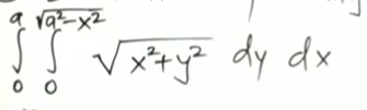
Thus, populating the Jacobian determinant :

We get $|J|$ = $r$.

But we have $dydx$ in our question, not $dxdy$.

So here we need to change the order of integration to correctly fit the replacement.

So we have $$y = \sqrt{a^2 - x^2}$$ as it's upper limit.

or $$y^2 = a^2 - x^2$$, or $$x^2 + y^2 = a^2$$

Which is the equation of a circle.

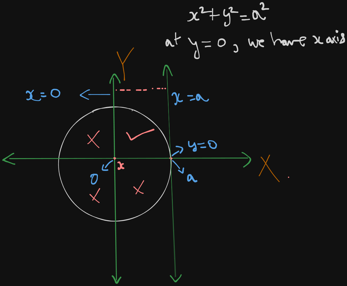
However, notice that we have $$y = \sqrt{a^2 - x^2}$$

the value of $y$ is positive. Which means we are concerned only with the upper half of the circle.

To narrow down the region further down, have our lines defined for $x=0$ and $x=a$.

Between these lines, the region which the equation covers, is the first quadrant only.

So this is the region for the circle :

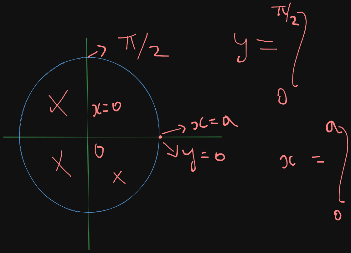
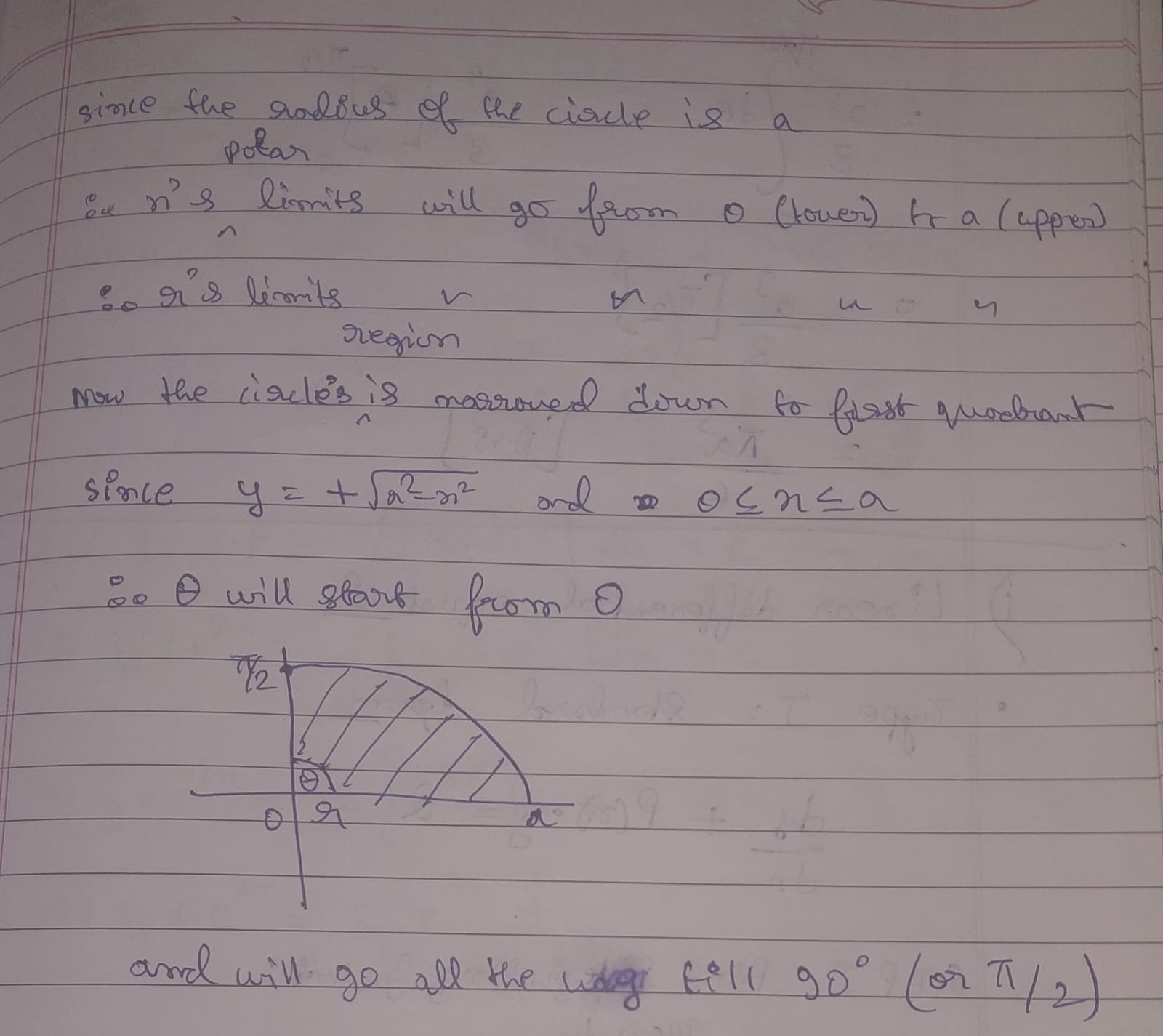
And now have the appropriate new limits as well as the limits for their polar counter-parts

So we can safely re-write the integral as :

And finally replace $dxdy$ to $rdrd\theta$

Thus our integral finally becomes,

Now we can solve this integral.

So $$\int_0^{\frac{\pi}{2}} \int_0^a {\sqrt{r^2cos^2\theta+r^2sin^2\theta}},r ,dr,d\theta$$
equals

or $$\int_0^{\frac{\pi}{2}} \int_0^a {\sqrt{r^2}},r ,dr,d\theta$$
or $$\int_0^{\frac{\pi}{2}} \int_0^a r ,. r ,dr,d\theta$$
or $$\int_0^{\frac{\pi}{2}} \int_0^a r^2 ,dr,d\theta$$
or $$\int_0^{\frac{\pi}{2}} [\frac{r^3}{3}]_0^a ,d\theta$$
or $$\frac{a^3}{3} \int_0^{\frac{\pi}{2}}d\theta$$
or $$\frac{a^3}{3} [\theta]_0^{\frac{\pi}{2}}$$
or $$\frac{\pi a^3}{6}$$

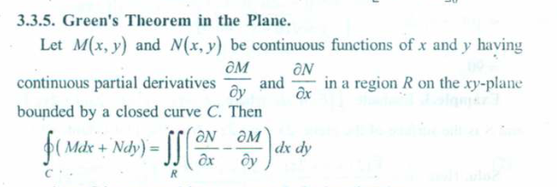
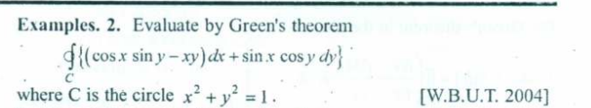
Green's Theorem (Statement only)

https://www.youtube.com/watch?v=8SwKD5_VL5o (since the embed can't be rendered in a PDF)

Here's a very cool visual explanation of Green's Theorem

or in another variant (a special case which actually becomes Stoke's Theorem)

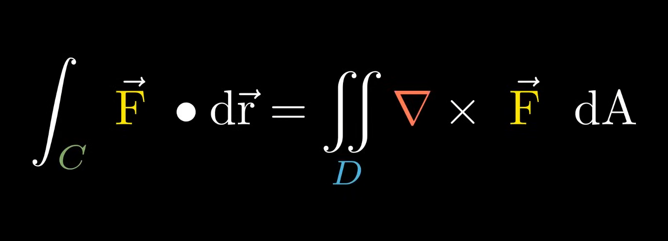
And here's the statement.

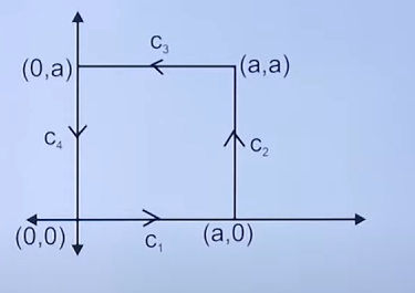
So let's say we have a curve C.

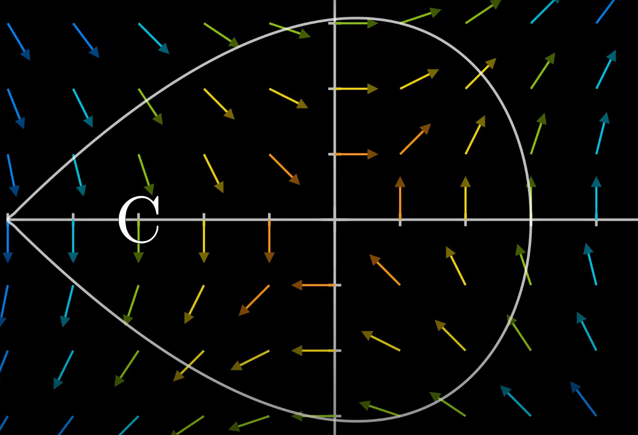
And we can call the region inside of this curve as R.

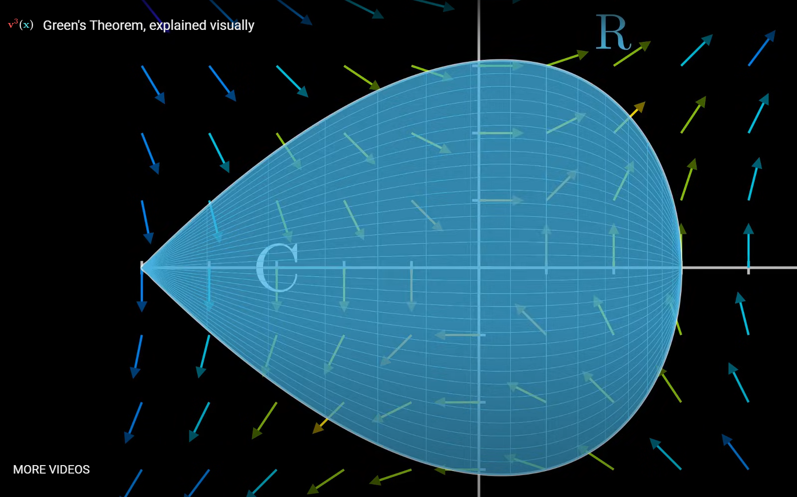
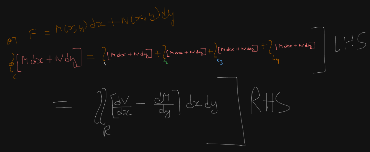
So Green's theorem states that the "The line integral of F over C is equal to the double integral of the 2-D curl of F over R".

What does this mean? What is a line integral?

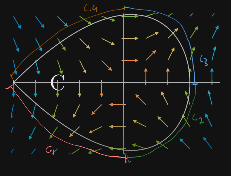
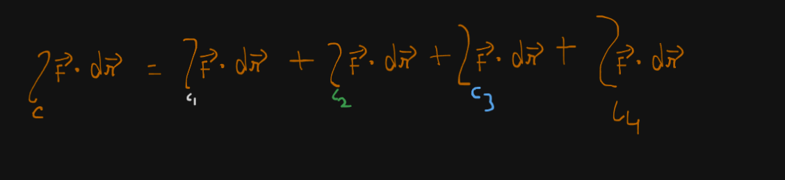
So let's say we divided the curve into 4 smaller "line curves" or just lines.

Naming them $c_1$, $c_2$, $c_3$, $c_4$, each.

Now the LHS side, the "line integral of F over C" would be given by finding the line integrals of all the smaller line curves and summing them up.

So we would get : $$\boxed{\int_c{F} \ dr = \int_{c_1}{F} \ dr \ + \int_{c_2}{F} \ dr + \ \int_{c_3}{F} \ dr + \ \int_{c_4}{F} \ dr} $$
where the surface C is traversed in the counter-clockwise direction.

And on the RHS.

Depending on what you have, two continuous functions M(x,y) and N(x,y) or a vector.

We have two equations :

In case of a vector :

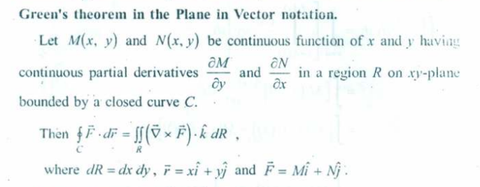
The curl of the vector F is the same as $\frac{dN}{dx}-\frac{dM}{dy}$ which we use if we have two continuous functions M and N.

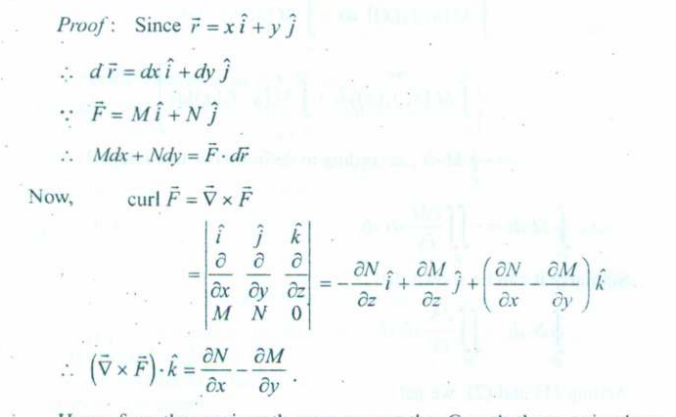
So in case of us having two continuous functions M and N, we have the RHS as :

Some solved examples.

Example 1.

Let's say we have to deal with this example where we are asked to verify Green's Theorem.

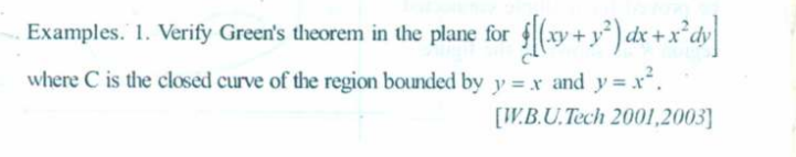
So we need to verify the LHS and RHS of Green's theorem

So here we have M = $xy+y^2$ and N = $x^2$

And we are given to curves, $y=x$ and $y=x^2$

So we can imagine $y=x^2$ as a parabolic line starting from the origin. And we the line $y=x$ as a line starting from the origin, going upward at a $45\mathrm{°}$ angle.

Let $C_1$ be the parabolic line $y=x^2$ and $C_2$ be for $y=x$.

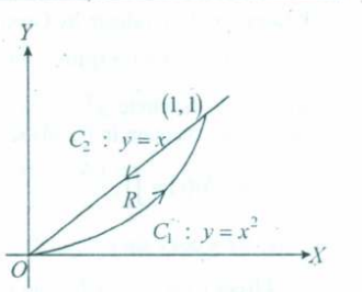
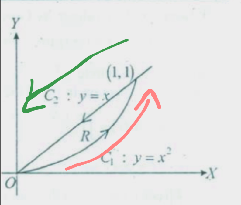
So we see that both the lines intersect at point (1,1).

The clockwise traversal will be like this :

So $$\int_c{[M \ dx \ + \ N \ dy]} = \int_{c_1} {[M \ dx \ + \ N \ dy]} \ + \ \int_{c_2} {[M \ dx \ + \ N \ dy]}$$

So, on $C_1$ we have $y=x^2$ . On differentiating both sides, we get : $dy=2xdx$
on $C_2$, we have $y=x$ . On differentiating both sides, we get: $dy=dx$

Why did we differentiate the both sides of these equations? So that during the solving of the line integral we get an easier calculation in terms of a single variable.

Limits for $C_1$ goes from origin (0,0) to point (1,1) so 0 to 1.

Limits for $C_2$ goes from point (1,1) back to origin (0,0), so 1 to 0.

Therefore we get : $$ \int_{c_1} {[M \ dx \ + \ N \ dy]} \ + \ \int_{c_2} {[M \ dx \ + \ N \ dy]} = \int_{0}^{1}{[xy + y^2 \ dx \ + x^2 \ dy]} + \int_{1}^{0}{[xy + y^2 \ dx \ + x^2 \ dy]}$$
substituting $y=x^2$ for $C_1$ and $y=x$ for $C_2$ and their respective $dy$ values.

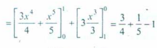
Now for the RHS.

We need to figure out : $$\int_R{\int_R{\frac{dN}{dx} - \frac{dM}{dy} \ dx} \ dy}$$
And for R. we have $x$ going from origin (0,0) to point(1,1), so 0 to 1.

And we already have y parameterized on x as in the given curves :

$y=x^2$ to $y=x$.

$\frac{dN}{dx}=2x$ and $\frac{dM}{dy}=x+2y$

$\therefore \frac{dN}{dx}-\frac{dM}{dy}=2x-(x+2y)=x-2y$

Note that we changed the order of integration from $dxdy$ to $dydx$ because of the how the limits were placed in the integral.

which is the same as our LHS.

Thus LHS = RHS and Green's theorem is verified!

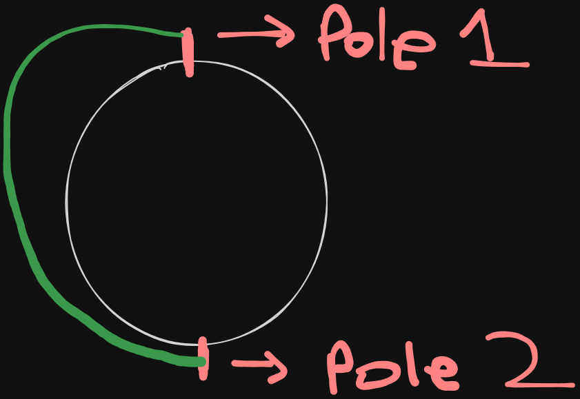
Example 2.

This is a pretty easy one. The question says "Evaluate" so we will only focus on finding the RHS here.

We have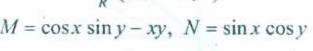

Thus

and

Since we are dealing with a circle here.

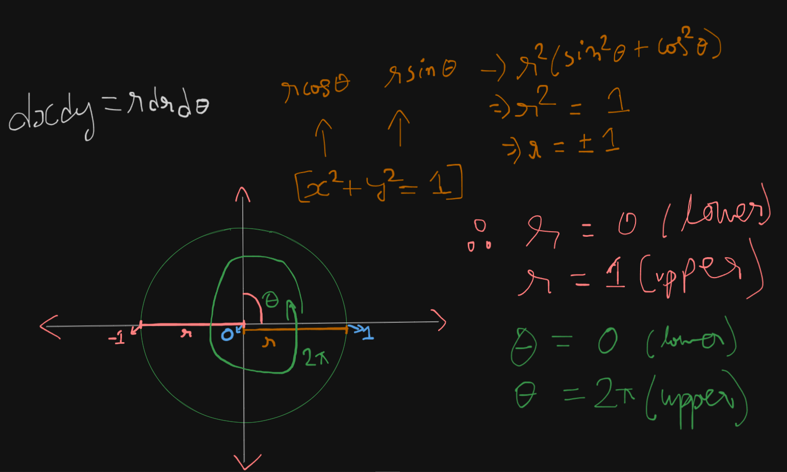
We will have to change $x$ to $rcos\theta$ for polar co-ordinates.

Thus $dxdy$ becomes $rdrd\theta$.

And the above picture states how we get the limits of r and $\theta$ .

There we get :

Thus we get zero as the answer for this one.

Gauss's Theorem (Statement only)

Here's a nice explanation video of Gauss's Theorem :

https://www.youtube.com/watch?v=zZqxbwl3Dno (since the embed can't be rendered in a PDF)

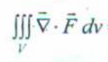
So The Divergence Theorem of Gauss states that the flux of whatever volume of fluid/electric field/electromagnetic field passing through either a surface or all the surfaces of a 3-D object can be given by :

where $\mathrm{\nabla }\cdot \mathbf{F}$ is the divergence of the vector F. Let's assume that :

Thus $$\nabla \cdot \mathbf{F} = \frac{d(x)}{dx} + \frac{d(y)}{dy} + \frac{d(z)}{dz}$$

Now to understand the RHS and how the $\hat{n}$ vector works, we need to understand the Surface Integral.

What is a Surface Integral?

https://www.youtube.com/watch?v=X2Z0tJG0rjU (since the embed can't be rendered in a PDF).

So a Surface Integral is basically any integral which is to be evaluated over a surface.

That surface could be any type.

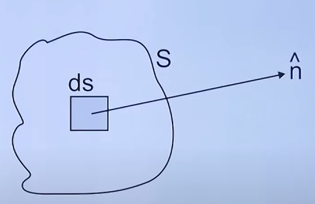
So here we have the surface S. The surface integral for this surface will be given by :

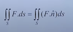
where the unit vector $\hat{n}$ is the vector normal to the surface S and pointing outwards.

Now there's a note we need to follow.

Depending on what plane the surface which we are dealing with is on :

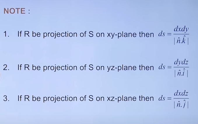
Thus,

XY plane : $\hat{n}=\hat{k}$
YZ plane: $\hat{n}=\hat{i}$
XZ plane: $\hat{n}=\hat{j}$

What is a plane?

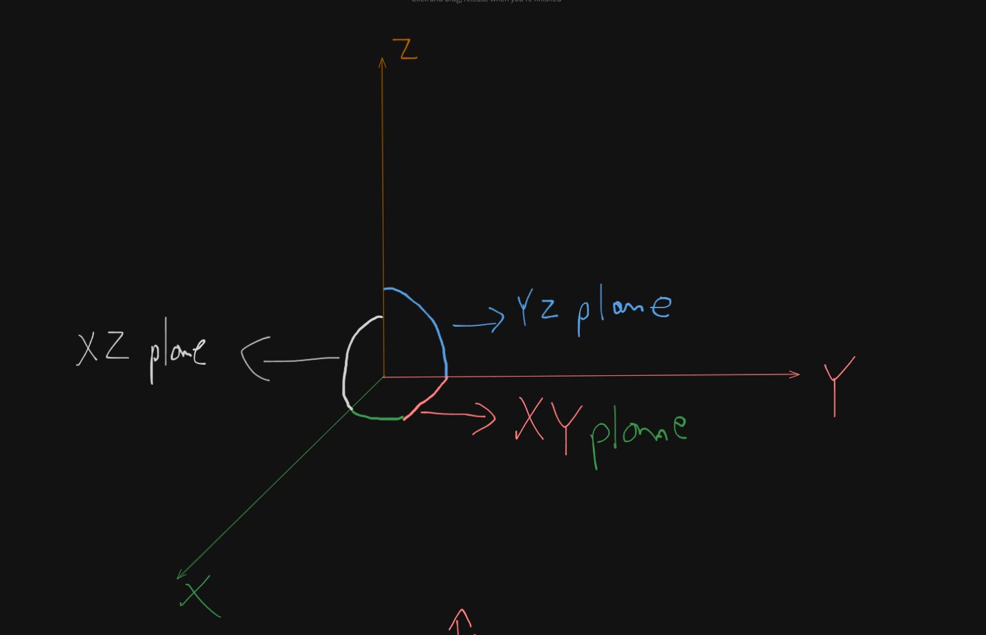
In the event where there is plane specified or you are given terms like "first quadrant" or "first octant", we will simply default to the x-y plane.

That's great, now how do we find the value of the unit normal vector, $\hat{n}$ ?

We can find that using this formula :

For vector $F=3x{y}^3-2x{z}^2$

And $$magnitude \ of \ gradient(F) = \sqrt{[{\frac{d(x)}{dx}]}^2 + {[\frac{d(y)}{dy}]}^2 + {[\frac{d(z)}{dz}]}^2}$$

Now watch the attached video for surface integral, the two examples in there should clear up any doubts regarding this.

Back to Gauss's theorem.

Let's solve two examples to better understand how Gauss's theorem works :

Example 1.

So we have been given a vector $F=4xz\hat{i}-y^2\hat{j}+yz\hat{k}$ and been given a 3-D cube's dimensions.

The resulting cube will be like this :

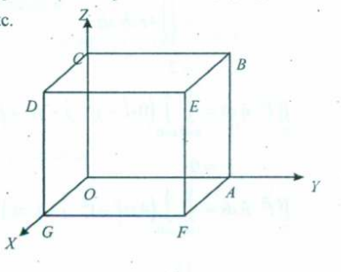
So first we need to find the LHS, which is :

so the divergence of vector F will be : $4z-2y+y=4z-y$.

Now we don't need to find the limits of V as it's been given pretty straightforward, all three, x, y and z go from 0 to 1.

The order of integration will be $dxdydz$.

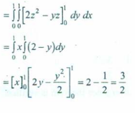
which will result in $$\frac{3}{2}$$

Now for the RHS, what we need to figure out is the flux of the volume through all the surfaces of this cube.

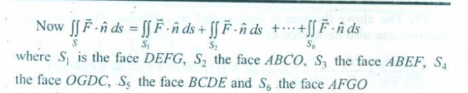
So for each face, we need to figure out what the $\hat{n}$ will be.

So what we did here was in each face, substitute the value of x, y or z.

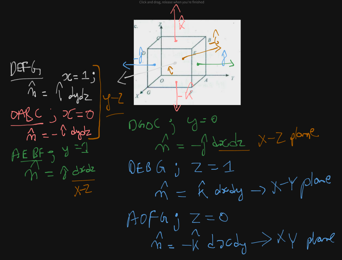
Using the rules for each plane from our picture earlier,

XY plane : $\hat{n}=\hat{k}$
YZ plane: $\hat{n}=\hat{i}$
XZ plane: $\hat{n}=\hat{j}$,

We figured out which face of the cube was parallel to which axes plane, and corresponding that we figured out the vector component, and each variable's value.

And thus we see that the RHS also has the same value as the LHS, $\frac{3}{2}$ and so Gauss's theorem is verified.

Example 2

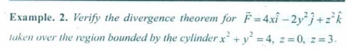
So first of all we need to verify the LHS.

So we have LHS as :

Now, so the divergence of vector F will be : $4-4y+2z=4-4y+2z$.

Now let's say we were to cut the cylinder like this:

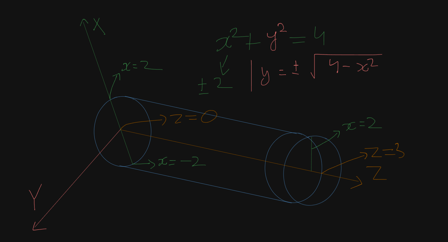
Each cross-section of the cylinder would result in a circle of radius x = 2.

Thus we get x = -2 (lower) to +2 (upper) from the equation of $x^2+y^2=4$.

Now for a fixed value of x, y can range from $-\sqrt{4-x^2}$ (lower) to $+\sqrt{4-x^2}$ (upper).

And we are already given that z goes from 0 to 3.

So now we can write :

Now eventually after solving this integral you will reach a step where you will have :

Now we will convert to polar coordinates, but instead of choosing $x=rcos\theta$, we will choose

$x=rsin\theta$ since otherwise LHS = RHS doesn't happen (I spent an entire day on this shit I know that it's right.)

and we already know that radius of the circle = 2.

Thus $$x = 2sin\theta$$
And so for $x=-2$

And for $x=2$

Differentiating for both sides :

Thus we get

Now for the RHS.

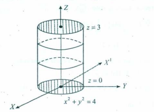
where $S_1$ is the circular base of the cylinder.
$S_2$ is the circular top of the cylinder.
$S_3$ is the curved surface of the cylinder given by $x^2+y^2=4$

For $S_1$, z = 0, the circle is on the XY plane, so $\hat{n}=-\hat{k}$.

For $S_2$, z = 3, the circle is parallel to the XY plane, so $\hat{n}=\hat{k}$

Now the surface goes along the XZ plane.

Therefore x will be set to $rcos\theta$ and $y=rsin\theta$

And $\theta$'s limits will go from 0 to $2\pi$ for the circular ends of the surface.

We already have z's limits.

The order of integration will be $rdzd\theta$, the $r$ being there because of the co-ordinate change.

So we will have

And on solving this ridiculously large integral we will get :

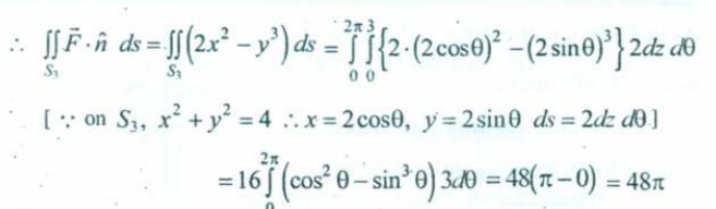
as the value for the third surface integral.

Adding them up, we get :

Thus, LHS = RHS and Gauss's Divergence theorem is verified!

Stokes's Theorem (Statement only)

Here's a nice explanation video on Stokes's Theorem

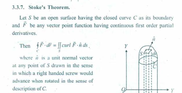
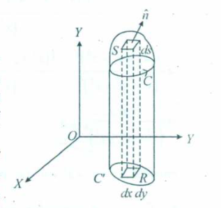
Or to explain it in a better way :

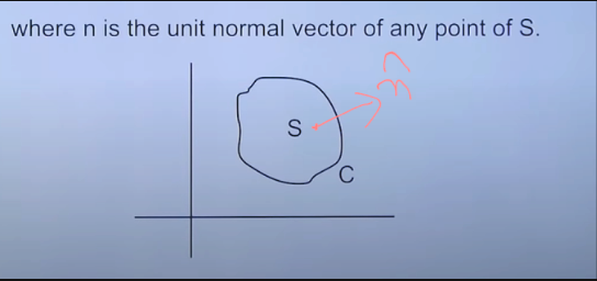
This is the special case for Green's Theorem

The curl of the vector F is the same as $\frac{dN}{dx}-\frac{dM}{dy}$ which we use if we have two continuous functions M and N.

However for Stoke's theorem we usually won't have two continuous functions M and N, instead we will have a vector field F.

Since we already dealt with Green's theorem and surface integrals, the process will be more or less similar.

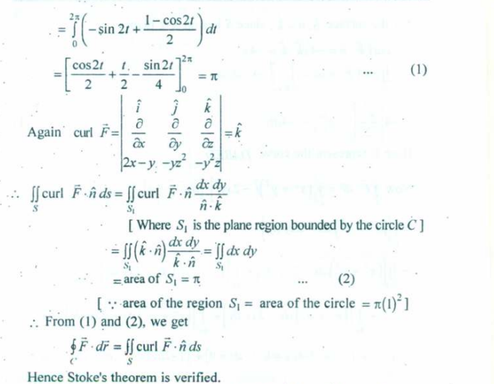
Example 1

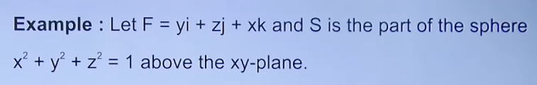
which is the same question as :

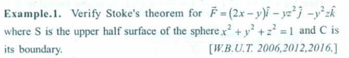
Note that the vectors given in the two questions are different but the equation is the same for the circle so we have the same diagrams in both questions :

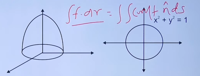
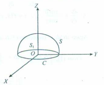
So, for the LHS :

which the line integral over the entire sphere's boundary, including the circle on the XY plane.

So we will get :

Now since we only concerned with the XZ plane, $z=0$ and $dz=0$

Thus,

Converting to polar co-ordinates,

$x=rcos\theta$ and $y=rsin\theta$ and $\theta$ will go from 0 to $2\pi$ since we are only dealing the circle here as the equation has changed from $x^2+y^2+z^2=1$ to $x^2+y^2=1$ which is the equation of a circle (as z = 0)

From the equation $$x^2 + y^2 = 1 \implies r^2 = 1 \implies r = \pm 1$$

However since we are concerned with the XY plane we will have r = 1.

Thus differentiating both sides of $x=rcos\theta$, we get $dx=1.-sin\theta d\theta$

Thus,

becomes :

and for the RHS here :

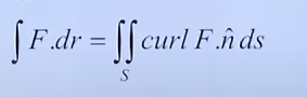
We need to find the curl of the given vector. Let's go with the vector in the example from the video as it's a simpler one.

Thus we get $$curl(F) = -\hat{i} - \hat{j} - \hat{k}$$
And what about the unit normal vector $\hat{n}$ ?

Since in both, the video and the book, we see that the sphere is sitting on the XY plane, from our rules :

XY plane : $\hat{n}=\hat{k}$
YZ plane: $\hat{n}=\hat{i}$
XZ plane: $\hat{n}=\hat{j}$,

We will have $\hat{n}=\hat{k}$. ( $+\hat{k}$ since the question explicitly says "above the XY plane", so the vector will point inwards of the sphere).

Thus,

And we are left with :

which is the formula of the area of a circle

Now if we set $x=rcos\theta$ and $y=rsin\theta$

From the equation $$x^2 + y^2 = 1 \implies r^2 = 1 \implies r = \pm 1$$

However since we are concerned with the XY plane we will have r = 1.

Thus ,

Thus LHS = RHS, and Stoke's theorem is verified!

For the vector given in the book, it was the same result, just was positive instead of negative.

Example 2:

The second example in the video :

is the same as :

however just with a different vector and shape, but contains 4 line integrals overall.

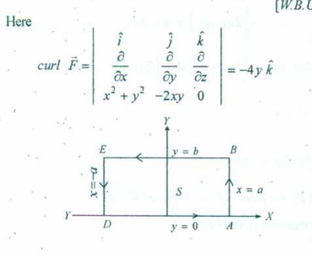
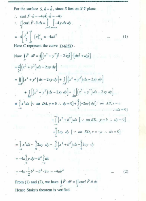
This is the solution for the book's problem. To understand this, watch the example 2 in the video as the procedure is the same more or less, like the previous question.