Important Questions (Organizer Included) -- Data Warehousing and Data Mining
Index
Module 2
What is the difference between Density-Based and Grid-Based Clustering?
Density-Based Clustering
Density-based clustering methods group together data points that are closely packed together (high density) and mark as outliers points that lie alone in low-density regions. Unlike partitioning methods like k-means, density-based methods don't require you to specify the number of clusters beforehand and can discover clusters of arbitrary shapes.
Key Idea: A cluster is a contiguous region of high point density, separated from other such regions by areas of low point density.
Core Concepts:
- Epsilon (
): A radius around a data point. - Minimum Points (MinPts): The minimum number of points required within the ϵ-neighborhood of a point to consider that point a core point.
- Core Point: A point that has at least
MinPtswithin its ϵ-neighborhood. - Border Point: A point that is not a core point but falls within the ϵ-neighborhood of a core point.
- Noise Point (Outlier): A point that is neither a core point nor a border point.
How it Works (using DBSCAN - Density-Based Spatial Clustering of Applications with Noise as a popular example):
- Start with an arbitrary unvisited point in the dataset.
- Retrieve its ϵ-neighborhood.
- If this neighborhood contains at least
MinPts, a new cluster is started, and all points in the neighborhood are added to this cluster. - Recursively visit and add their ϵ-neighborhoods to the cluster if they are also core points.
- If the initial point has fewer than
MinPtsin its ϵ-neighborhood, it's temporarily labeled as noise. This noise point might later become part of a cluster if it's within the ϵ-neighborhood of a core point. - This process continues until all points have been visited.
Advantages of Density-Based Clustering:
- Can discover clusters of arbitrary shapes.
- Handles outliers well.
- Doesn't require specifying the number of clusters in advance.
Disadvantages:
- Can have trouble with clusters of varying densities.
- Performance can degrade in high-dimensional spaces.
- The choice of ϵ and
MinPtscan significantly affect the results.
Grid-Based Clustering
Grid-based clustering methods quantize the data space into a finite number of cells (forming a grid structure) and then perform clustering on these grid cells. The main advantage is their speed, as the clustering is done on the grid, which is usually much smaller than the number of data points.
Key Idea: Divide the data space into a grid of cells and then identify dense cells to form clusters.
General Approach:
- Grid Creation: Divide the data space into a grid of cells. The granularity of the grid can affect the quality of the clustering.
- Cell Density Calculation: For each cell, calculate the number of data points that fall within it (the density of the cell).
- Cluster Formation: Merge adjacent dense cells to form clusters. The definition of "dense" (based on a threshold) and "adjacent" needs to be specified.
Example Algorithms:
- STING (Statistical Information Grid): Divides the spatial area into rectangular cells at different resolution levels, forming a hierarchical structure. Statistical information (like mean, min, max, distribution) is stored in each cell, which is used for query processing and clustering.
- CLIQUE (CLustering In QUEst): A subspace clustering algorithm that combines density-based and grid-based approaches. It identifies dense regions in subspaces of high dimensionality.
- WaveCluster: Uses wavelet transform to cluster data points by multi-resolution analysis.
Advantages of Grid-Based Clustering:
- Generally very fast processing time, often independent of the number of data objects (dependent on the number of grid cells).
- Easy to implement.
- Can handle large datasets efficiently.
Disadvantages:
- The quality of the clustering depends on the granularity of the grid. Too coarse a grid might merge distinct clusters, while too fine a grid might break up natural clusters.
- Can have difficulty with high-dimensional data due to the exponential increase in the number of grid cells.
- The shape of the clusters is somewhat restricted by the grid structure.
State the four axioms of distance metrics
A "distance metric" (or simply "metric") is a function that defines a distance between elements of a set, satisfying certain intuitive properties. These properties are often called the four axioms of a distance metric.
The Four Axioms of Distance Metrics:
-
Non-negativity:
: The distance between any two points must always be non-negative. You can't have a negative distance. -
Identity of Indiscernibles (or Reflexivity):
: The distance between two points is zero if and only if the points are identical. If the distance is zero, they're the same point, and if they're the same point, their distance is zero. -
Symmetry:
: The distance from point x to point y is the same as the distance from point y to point x. The order of the points doesn't matter. -
Triangle Inequality:
: For any three points , and , the direct distance between x and z must be less than or equal to the sum of the distances from x to y and from y to z. In simpler terms, the shortest path between two points is a straight line, and taking a detour through a third point will never make the journey shorter.
Difference between CLARA/CLARANS methods and how to perform clustering with the methods.
CLARA (Clustering LARge Applications)
CLARA was one of the first sampling-based clustering algorithms designed to handle large datasets that couldn't fit into memory. It's an extension of the K-Medoids (PAM - Partitioning Around Medoids) algorithm.
The Problem with K-Medoids/PAM: K-Medoids works by iteratively selecting data points as "medoids" (representative objects) and then assigning all other data points to their closest medoid. The objective is to minimize the sum of dissimilarities between points and their assigned medoids. However, K-Medoids has a time complexity of
How CLARA Solves It (using sampling)
CLARA addresses this by working on multiple random samples of the original dataset, rather than the entire dataset.
- Draw a Sample: From the huge dataset, CLARA draws a small random sample (e.g., 40 + 2k points, where k is the number of clusters).
- Apply K-Medoids: It then applies the K-Medoids (PAM) algorithm to this sample to find k medoids.
- Calculate Quality: Once the medoids are found from the sample, CLARA assigns all objects in the entire original dataset to their closest medoid. The quality of these medoids (e.g., the average dissimilarity) is then calculated over the entire dataset.
- Repeat and Choose Best: This process (sampling, K-Medoids on sample, calculating quality on full dataset) is repeated multiple times. CLARA then selects the set of medoids that yielded the best clustering (lowest average dissimilarity) over the entire dataset.
Advantages of CLARA:
- Can handle much larger datasets than K-Medoids.
- Significantly reduces computation time for large n.
Disadvantages:
- The quality of the clustering is highly dependent on the quality of the random sample. If a bad sample is chosen (i.e., not representative of the full dataset), the resulting medoids might not be optimal for the overall dataset.
CLARANS (Clustering Large Applications based upon RANdomized Search)
CLARANS is an improvement over CLARA, also designed for large datasets, but it uses a randomized search approach instead of just sampling the data points. While CLARA performs K-Medoids on a fixed sample, CLARANS conducts a randomized search for optimal medoids in the graph of possible medoid sets.
The Problem with CLARA (potential for non-representative samples): As mentioned, CLARA's effectiveness hinges on the chosen samples being representative. If they're not, the final clustering might be suboptimal.
How CLARANS Solves It (randomized graph search):
Instead of selecting a single sample and running PAM on it, CLARANS works more like a search algorithm on the actual medoid combinations:
- Start Randomly: It starts with an arbitrary set of k medoids from the dataset.
- Define Neighborhood: It defines a "neighbor" of the current set of medoids as a set where only one medoid has been swapped with a non-medoid object.
- Randomized Local Search: CLARANS then randomly checks a predefined number of neighbors (
max_neighbors). If a neighbor set yields a better clustering (lower cost), it moves to that neighbor set and continues the search from there. - Local Optima: If after checking
max_neighborsit doesn't find a better neighbor, it assumes it has reached a "local optimum" and terminates this search process. - Multiple Iterations: This entire process (from a random start to a local optimum) is repeated a predefined number of times (
num_local). The best set of medoids found across all these local searches is chosen as the final result.
Advantages of CLARANS:
- More effective than CLARA at finding better quality clusterings because it explores the search space of medoids more thoroughly (though randomly).
- Can overcome the problem of "bad samples" that CLARA might encounter.
Disadvantages:
- Still computationally more expensive than CLARA, although less than K-Medoids for very large N.
- Requires tuning of
max_neighborsandnum_localparameters.
Example
(No need of going over this if it feels too confusing)
Let's imagine applying a medoid-based algorithm like K-Medoids (which CLARA/CLARANS use internally) to this dataset [(2, 3), (4, 5), (6, 7)] . For simplicity, let's assume we want to find k=2 clusters.
P1=(2,3), P2=(4,5), P3=(6,7)
Since the dataset is tiny, CLARA/CLARANS wouldn't typically be used for it, but the concept of finding medoids applies.
Step-by-step (conceptual K-Medoids):
-
Initial Medoid Selection: Let's randomly choose two points as initial medoids. Suppose we pick:
- Medoid 1 (M1) = P1=(2,3)
- Medoid 2 (M2) = P2=(4,5)
-
Assign Points to Closest Medoids: We'll use Manhattan distance for simplicity.
-
For P1=(2,3):
- Distance to M1=(2,3):
- Distance to M2=(4,5):
- P1 is closest to M1. Cluster 1:
- Distance to M1=(2,3):
-
For P2=(4,5):
- Distance to M1=(2,3):
- Distance to M2=(4,5):
- P2 is closest to M2. Cluster 2:
- Distance to M1=(2,3):
-
For P3=(6,7):
- Distance to M1=(2,3):
- Distance to M2=(4,5):
- P3 is closest to M2. Cluster 2:
- Distance to M1=(2,3):
Current Clusters:
- Cluster 1 (Medoid M1):
- Cluster 2 (Medoid M2):
Current Cost (Sum of Dissimilarities):
- Cost =
- Cost = 0+0+4=4
-
-
Update Medoids (Iterate): Now, K-Medoids (and by extension CLARA/CLARANS) would try to improve the clustering by swapping medoids with non-medoid points.
Let's consider swapping M1=(2,3) with P3=(6,7) (the only non-medoid point in the first cluster). This isn't really applicable here as P1 is the only point in its cluster. The next step would be to try swapping M1 or M2 with a non-medoid point to see if the cost improves.
Let's try swapping M1=(2,3) with P3=(6,7). New Medoids: M1′=(6,7), M2=(4,5)
-
For P1=(2,3):
- Distance to M1′=(6,7):
- Distance to M2=(4,5):
- P1 is closest to M2.
- Distance to M1′=(6,7):
-
For P2=(4,5):
- Distance to M1′=(6,7):
- Distance to M2=(4,5): 0
- P2 is closest to M2.
- Distance to M1′=(6,7):
-
For P3=(6,7):
- Distance to M1′=(6,7): 0
- Distance to M2=(4,5): 4
- P3 is closest to M1′.
New Clusters:
- Cluster 1 (Medoid M1′):
- Cluster 2 (Medoid M2):
New Cost:
- Cost =
d(P3,M1′)+d(P1,M2)+d(P2,M2) - Cost = 0+4+0=4
In this particular very small example, the cost remained the same. An algorithm like K-Medoids (and thus CLARA/CLARANS at their core) would continue to explore swaps until no further improvement in cost can be made, reaching a local optimum. Given the simplicity of the dataset, it's likely to quickly converge.
-
Reservoir Sampling in Data Stream Mining
Imagine you're watching a never-ending conveyor belt of items, and you want to pick a random sample of, say, 5 items from everything that passes by. You can't wait for the conveyor belt to end because it never does, and you don't have enough space to store all the items. This is where reservoir sampling comes in.
The Problem: Sampling from a Data Stream
In traditional sampling, if you have a finite list of N items, and you want to pick k random items, you could simply generate k random indices between 1 and N and pick those items. But with a data stream:
- Unknown Size: You don't know N (the total number of items) beforehand. The stream might be infinite, or just very, very long.
- Single Pass: You can't store the entire stream. You process items one by one.
- Uniform Probability: You want every item that has passed through the stream to have an equal chance of being in your final sample.
Reservoir Sampling (Algorithm R) - The Easy Explanation
Let's say you want to maintain a random sample of k items. You'll keep these k items in a small "reservoir" (think of it as a small bucket).
Here's how it works:
-
Fill the Reservoir: Take the first
kitems that arrive from the stream and put them directly into your reservoir. Your reservoir is now full. -
Process Subsequent Items: For every new item that arrives after the first
k(let's say the current item is thei-thitem, where): - Generate a random number
jbetween1andi(inclusive). - If
jis less than or equal tok: This means the new item "wins" a spot in the reservoir. You replace a random item currently in the reservoir (specifically, the item at indexj-1if your reservoir is 0-indexed) with the newi-thitem. - If
jis greater thank: The new item is discarded, and the reservoir remains unchanged.
- Generate a random number
Example
Let's assume:
irepresents the 1-based count of the current item from the stream.- The reservoir is a 0-indexed array of size
k. - We want to sample k=2 items from a stream.
Initial Reservoir: reservoir = [None, None] (size 2, initially empty)
Stream of items: A, B, C, D, E, F, ...
1. Process Item A (1st item, i=1):
i(1) ≤k (2). Fill reservoir.reservoir[0] = A- Reservoir:
[A, None]
2. Process Item B (2nd item, i=2):
i(2) ≤k (2). Fill reservoir.reservoir[1] = B- Reservoir:
[A, B](Reservoir is now full)
3. Process Item C (3rd item, i=3):
i(3) >k (2). Apply the replacement logic.- Generate a random number
jbetween 1 andi(which is 3). Sojcan be 1, 2, or 3. - Let's say
j = 2. - Condition Check: If
j(2) ≤k (2). This is true. - Replacement: Replace
reservoir[j-1]with the new item. Sincej=2, we replacereservoir[1]withC. - Reservoir:
[A, C]
4. Process Item D (4th item, i=4):
i(4) >k (2). Apply the replacement logic.- Generate a random number
jbetween 1 andi(which is 4). Sojcan be 1, 2, 3, or 4. - Let's say
j = 4. - Condition Check: If
j(4) ≤k (2). This is false. - Action: Discard D. Reservoir remains unchanged.
- Reservoir:
[A, C]
5. Process Item E (5th item, i=5):
i(5) >k (2). Apply the replacement logic.- Generate a random number
jbetween 1 andi(which is 5). Sojcan be 1, 2, 3, 4, or 5. - Let's say
j = 1. - Condition Check: If
j(1) ≤k (2). This is true. - Replacement: Replace
reservoir[j-1]with the new item. Sincej=1, we replacereservoir[0]withE. - Reservoir:
[E, C]
6. Process Item F (6th item, i=6):
i(6) >k (2). Apply the replacement logic.- Generate a random number
jbetween 1 andi(which is 6). Sojcan be 1, 2, 3, 4, 5, or 6. - Let's say
j = 5. - Condition Check: If
j(5) ≤k (2). This is false. - Action: Discard F. Reservoir remains unchanged.
- Reservoir:
[E, C]
When is it Used?
- Log Analysis: Sampling a subset of log entries from a continuously flowing stream of server logs.
- Network Monitoring: Sampling packets for traffic analysis without storing all of them.
- Sensor Data: Collecting a representative sample from a never-ending stream of sensor readings.
- Online Analytics: Providing approximate answers to queries on massive, live datasets where storing everything is impossible.
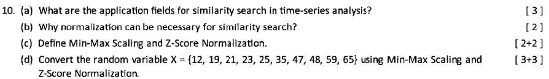
(a) What are the application fields for similarity search in time-series analysis? [3 marks]
Answer:
Similarity search in time-series analysis involves finding sequences that are similar to a given time-series pattern. This is useful in various fields, including:
- Finance: Identifying similar stock price patterns to predict future trends or detect anomalies (e.g., market crashes).
- Healthcare: Comparing patient data, like ECG or heart rate time-series, to detect abnormalities or match symptoms to known conditions.
- Weather Forecasting: Finding historical weather patterns that match current conditions to predict future weather events.
These applications help in pattern recognition, anomaly detection, and predictive modeling.
(b) Why normalization can be necessary for similarity search? [2 marks]
Answer:
Normalization is often necessary for similarity search in time-series analysis because:
- Scale Differences: Time-series data may have different scales (e.g., one series in the range
[0, 100]and another in[0, 1000]). Without normalization, the larger-scale series will dominate similarity measures like Euclidean distance, leading to inaccurate comparisons. - Offset Variations: Time-series may have different baselines or offsets (e.g., one series starts at 50, another at 500). Normalization adjusts for these shifts, ensuring the focus is on the shape of the series rather than absolute values.
Normalization ensures that similarity is based on the patterns and trends in the data, not on their raw magnitudes or offsets.
(c) Define Min-Max Scaling and Z-Score Normalization. [2+2 marks]
Let’s break this down clearly since this is one of the topics we haven’t explored before.
Min-Max Scaling
Min-Max Scaling transforms the data into a fixed range, typically [0, 1], by rescaling the values based on the minimum and maximum values in the dataset. The formula is:
: Original value : Minimum value in the dataset : Maximum value in the dataset : Scaled value (between 0 and 1)
This method preserves the shape of the data distribution but adjusts the range. It’s useful when you need data in a specific range for similarity comparisons or machine learning models.
Z-Score Normalization
Z-Score Normalization (also called standardization) transforms the data to have a mean of 0 and a standard deviation of 1. The formula is:
: Original value : Mean of the dataset : Standard deviation of the dataset : Normalized value
This method makes the data distribution centered around 0 with a standard deviation of 1, which is helpful for similarity search because it removes the effect of scale and focuses on how far each point is from the mean in terms of standard deviations.
Key Difference: Min-Max Scaling bounds the data to a specific range (e.g., [0, 1]), while Z-Score Normalization adjusts the data based on its statistical properties (mean and standard deviation), and the resulting values are not bound to a specific range.
(d) Convert the random variable [3+3 marks]
Consider this an example to Min-Max Scaling and Z-Score Normalization.
So let's lay out the dataset in a tabular format.
| X |
|---|
| 12 |
| 19 |
| 21 |
| 23 |
| 25 |
| 35 |
| 47 |
| 48 |
| 59 |
| 65 |
Min-Max Scaling
Formula for Min-Max Scaling:
Let's start then.
| X | ||||
|---|---|---|---|---|
| 12 | 12 | 65 | 53 | |
| 19 | 12 | 65 | 53 | 0.1320 |
| 21 | 12 | 65 | 53 | 0.1698 |
| 23 | 12 | 65 | 53 | 0.2075 |
| 25 | 12 | 65 | 53 | 0.2452 |
| 35 | 12 | 65 | 53 | 0.4339 |
| 47 | 12 | 65 | 53 | 0.6603 |
| 48 | 12 | 65 | 53 | 0.6792 |
| 59 | 12 | 65 | 53 | 0.8867 |
| 65 | 12 | 65 | 53 | 1 |
Min-Max Scaled Values (rounded to 4 decimal places):
Z-Score Normalization
Formula for Z-Score Normalization
So, we have the dataset as:
| X |
|---|
| 12 |
| 19 |
| 21 |
| 23 |
| 25 |
| 35 |
| 47 |
| 48 |
| 59 |
| 65 |
Let's start then.
For standard deviation we need the variance first:
And the standard deviation is the square root of the variance.
where
| X | ||||
|---|---|---|---|---|
| 12 | 35.4 | 547.56 | -1.3482 |
|
| 19 | 35.4 | 268.96 | 17.3562 | -0.9449 |
| 21 | 35.4 | 207.36 | 17.3562 | -0.8296 |
| 23 | 35.4 | 153.76 | 17.3562 | -0.7144 |
| 25 | 35.4 | 108.16 | 17.3562 | -0.5991 |
| 35 | 35.4 | 0.16 | 17.3562 | -0.0230 |
| 47 | 35.4 | 134.56 | 17.3562 | 0.6682 |
| 48 | 35.4 | 158.76 | 17.3562 | 0.7259 |
| 59 | 35.4 | 556.96 | 17.3562 | 1.3597 |
| 65 | 35.4 | 876.16 | 17.3562 | 1.7056 |
| Total | __ | 3012.4 | __ | __ |
Z-Score Normalized Values (rounded to 4 decimal places):
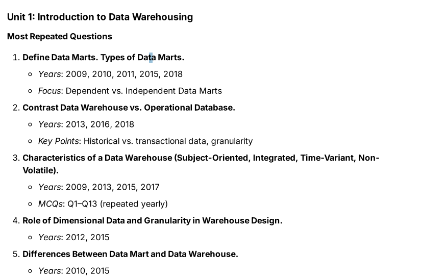
2024 paper Group C
Question 7
(a) What are some recent advancements in distributed warehousing technologies, and how do they impact data mining operations?
Answer:
Recent Advancements in Distributed Warehousing Technologies:
Distributed warehousing has evolved to handle large-scale data efficiently. Some recent advancements include:
- Cloud-Based Data Warehouses: Platforms like Snowflake, Google BigQuery, and Amazon Redshift enable scalable, on-demand storage and compute resources, reducing infrastructure costs and allowing global access.
- Data Lakehouse Architecture: Combining data lakes and warehouses (e.g., Delta Lake, Databricks), this approach supports structured and unstructured data in a single system, enabling more flexible data mining workflows.
- Federated Query Processing: Tools like Presto and Apache Drill allow querying across distributed systems without data movement, improving speed and reducing latency for data mining tasks.
Impact on Data Mining Operations:
-
Scalability: Cloud-based solutions allow data mining algorithms to scale with growing datasets, processing petabytes of data efficiently.
-
Speed: Federated queries and parallel processing reduce the time needed for data retrieval and preprocessing, speeding up mining tasks like frequent pattern mining or clustering.
-
Cost Efficiency: Pay-as-you-go models in cloud warehousing lower the cost of running resource-intensive mining operations.
-
Accessibility: Distributed systems enable real-time data mining across global teams, supporting applications like trend analysis or anomaly detection in dynamic environments.
(b) Discuss the role of ensemble learning methods in addressing the class imbalance problem.
Answer:
Class Imbalance Problem: (Already covered in module 4)
Class imbalance occurs when one class (e.g., the majority class) has significantly more instances than another (e.g., the minority class), common in datasets like fraud detection where fraudulent cases are rare. This skew can lead to biased models that favor the majority class, reducing accuracy for the minority class.
Role of Ensemble Learning Methods:
Ensemble learning combines multiple models to improve prediction performance and is effective for addressing class imbalance:
-
Bagging with Resampling: Techniques like Balanced Random Forest use bagging (Bootstrap Aggregating) with undersampling of the majority class or oversampling of the minority class in each bootstrap sample, ensuring balanced training data for each model.
-
Boosting with Weight Adjustments: Algorithms like AdaBoost or SMOTEBoost assign higher weights to minority class instances during training, focusing the model on harder-to-classify examples.
-
Hybrid Ensembles: Methods like EasyEnsemble create multiple balanced subsets of the data, train separate classifiers on each, and combine their predictions, improving minority class detection.
Benefits:
- Ensemble methods reduce bias toward the majority class by balancing the influence of each class.
- They improve overall model robustness and accuracy, especially for minority class predictions, which is critical in applications like medical diagnosis or fraud detection.
(c) How does graph mining contribute to anomaly detection in network data?
Answer:
Graph Mining Overview:
Graph mining involves analyzing graph-structured data (e.g., nodes and edges representing entities and relationships) to uncover patterns, communities, or anomalies. In network data, graphs represent entities like users, devices, or transactions, with edges showing interactions.
Contribution to Anomaly Detection:
- Structural Analysis: Graph mining identifies unusual structures, such as nodes with unexpected degrees (e.g., a user with too many connections in a social network, indicating a bot).
- Community Detection: Algorithms like Louvain or Spectral Clustering detect communities in networks; nodes that don’t belong to any community or have abnormal cross-community connections may be anomalies (e.g., a device in a network behaving differently).
- Path and Subgraph Analysis: Mining frequent subgraphs or shortest paths can reveal anomalies, such as unusual transaction patterns in a financial network indicating fraud.
Example:
In a cybersecurity network, graph mining can detect an anomaly if a device (node) suddenly connects to many others (high degree) or forms a subgraph with unusual patterns, suggesting a potential attack.
Question 9
(a) Discuss the challenges associated with mining transactional patterns in large-scale datasets.
Answer:
Overview of Transactional Pattern Mining:
Transactional pattern mining involves identifying frequent patterns in transactional datasets, such as items frequently purchased together (e.g., market basket analysis) or sequences of transactions (e.g., customer purchase sequences). In large-scale datasets, this process faces several challenges:
-
Scalability and Computational Complexity:
-
Large-scale datasets often contain millions of transactions, each with numerous items. Algorithms like Apriori or FP-Growth require multiple scans of the dataset to compute frequent itemsets, leading to high computational costs.
-
The number of possible item combinations grows exponentially (combinatorial explosion), making it infeasible to compute all patterns in memory or within reasonable time.
-
-
Memory Constraints:
- Storing the entire dataset and intermediate results (e.g., candidate itemsets in Apriori or the FP-tree in FP-Growth) in memory can be challenging. For example, in Apriori, the candidate generation step produces a large number of itemsets, which may exceed available memory in large datasets.
-
Sparsity and Noise:
-
Transactional datasets are often sparse (e.g., a customer buys only a few items out of thousands available), making it harder to find meaningful patterns.
-
Noise, such as irrelevant or erroneous transactions (e.g., data entry errors), can lead to the discovery of false patterns, reducing the quality of results.
-
-
Pattern Redundancy:
- In large datasets, many discovered patterns may be redundant or trivial (e.g., "if milk, then bread" might appear in many forms). Filtering out redundant patterns while preserving meaningful ones is computationally expensive and requires additional post-processing.
-
Distributed Data Handling:
- In large-scale systems, data is often distributed across multiple nodes (e.g., in cloud environments). Coordinating mining across distributed systems introduces challenges like data partitioning, communication overhead, and ensuring consistency in pattern discovery.
-
Dynamic Updates:
- Transactional data in large-scale systems is often dynamic (e.g., new purchases are added in real-time). Updating the mined patterns incrementally without re-running the entire mining process on the updated dataset is complex and resource-intensive.
-
Support Threshold Selection:
- Choosing an appropriate minimum support threshold is tricky. A low threshold generates too many patterns, increasing computational load, while a high threshold may miss important but less frequent patterns (e.g., rare but high-value purchases).
-
Interpretability and Actionability:
- With large datasets, the sheer volume of discovered patterns can overwhelm users. Ensuring that the mined patterns are interpretable and actionable for decision-making (e.g., in retail or marketing) requires additional effort, such as pattern summarization or ranking.
Mitigation Strategies:
-
Use scalable algorithms like FP-Growth, which avoids candidate generation, or parallelized versions like Parallel FP-Growth (PFP) for distributed systems.
-
Apply sampling or data partitioning to reduce the dataset size while preserving key patterns.
-
Use constraint-based mining to focus on specific patterns (e.g., high-value items) and reduce redundancy.
This addresses challenges in the context of Topic 1: "Sequential Pattern Mining concepts, primitives, scalable methods," which includes transactional pattern mining as a related concept.
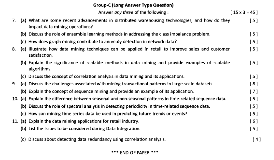
(b) Explain the concept of sequence mining and provide an example of its application.
Answer:
Sequence: A sequence is formally defined as the ordered set of items {s1, s2, s3, …, sn}. As the name suggests, it is the sequence of items occurring together. It can be considered as a transaction or purchased items together in a basket.
Subsequence: The subset of the sequence is called a subsequence. Suppose {a, b, g, q, y, e, c} is a sequence. The subsequence of this can be {a, b, c} or {y, e}. Observe that the subsequence is not necessarily consecutive items of the sequence. From the sequences of databases, subsequences are found from which the generalized sequence patterns are found at the end.
Sequence pattern: A sub-sequence is called a pattern when it is found in multiple sequences. For example: the pattern <a, b> is a sequence pattern mined from sequences {b, x, c, a}, {a, b, q}, and {a, u, b}.
-
Sequence Pattern Mining:
This focuses on identifying patterns that occur in a specific sequence over time, such as website click-streams or customer purchase sequences.
-
Algorithms: Common algorithms for sequence mining include GSP (Generalized Sequential Patterns), PrefixSpan, and SPADE, which differ in how they generate and evaluate candidate sequences.
-
Process:
- Represent the data as sequences (e.g., customer transactions over time).
- Define a minimum support threshold.
- Use an algorithm to find all frequent subsequences (e.g., PrefixSpan projects the database into smaller subsets to efficiently find patterns).
- Post-process the results to filter or rank patterns for actionability.
Application in E-Commerce (Customer Purchase Behavior):
Consider an e-commerce platform analyzing customer purchase sequences to recommend products. The dataset contains sequences of customer purchases over time:
Application:
The e-commerce platform can use the frequent subsequence
Question 10
(a) Explain the difference between seasonal and non-seasonal patterns in time-related sequence data.
Time-related sequence data, or time-series data, consists of observations recorded over time, often at regular intervals (e.g., daily sales, hourly temperature). Patterns in such data can be broadly classified into seasonal and non-seasonal patterns.
Seasonal Patterns:
-
Definition: Seasonal patterns are recurring, predictable variations in the data that occur at regular intervals due to seasonal factors. These intervals are often tied to natural or calendar cycles (e.g., daily, monthly, yearly).
-
Characteristics:
- Fixed periodicity: The pattern repeats at a consistent frequency (e.g., every 12 months for yearly seasonality).
- Often driven by external factors like weather, holidays, or cultural events.
-
Example: Retail sales often show a seasonal pattern with peaks during the holiday season (e.g., November–December) each year due to increased consumer spending. A time-series of monthly sales might show a spike every December.
Non-Seasonal Patterns:
-
Definition: Non-seasonal patterns are trends or variations in the data that do not follow a fixed, recurring cycle. These can include long-term trends, irregular fluctuations, or one-time events.
-
Characteristics:
- Lack of fixed periodicity: Changes are not tied to a regular interval.
- May include trends (e.g., a gradual increase or decrease over time) or random noise (e.g., unpredictable fluctuations).
-
Example: A company’s sales might show a non-seasonal upward trend over several years due to improved marketing strategies or market expansion, without any repeating cycle. Alternatively, a sudden drop in sales due to a one-time event (e.g., a supply chain disruption) is also non-seasonal.
Key Differences:
-
Periodicity: Seasonal patterns have a fixed, repeating cycle (e.g., every month or year), while non-seasonal patterns do not follow a regular cycle.
-
Predictability: Seasonal patterns are predictable based on historical cycles (e.g., higher ice cream sales in summer), whereas non-seasonal patterns may be less predictable (e.g., a sudden sales drop due to an economic crisis).
-
Cause: Seasonal patterns are often tied to external cycles (e.g., seasons, holidays), while non-seasonal patterns may result from long-term trends, random events, or structural changes.
-
Analysis Approach: Seasonal patterns are often analyzed using methods like seasonal decomposition (e.g., STL decomposition) to isolate the seasonal component, while non-seasonal patterns are studied using trend analysis or smoothing techniques (e.g., moving averages).
Illustration:
Consider a time-series of daily temperatures over several years:
-
Seasonal Pattern: Temperatures rise in summer (June–August) and fall in winter (December–February) each year, repeating annually.
-
Non-Seasonal Pattern: A gradual increase in average temperatures over decades due to climate change represents a long-term trend, not tied to a seasonal cycle.
(b) Discuss the role of spectral analysis in detecting periodicity in time-related sequence data.
Answer:
Overview of Spectral Analysis:
Spectral analysis is a technique used to analyze time-series data by transforming it from the time domain into the frequency domain. It helps identify periodic components (repeating patterns) in the data by examining the frequencies at which the data oscillates. This is particularly useful for detecting periodicity in time-related sequence data.
Role of Spectral Analysis in Detecting Periodicity:
-
Frequency Decomposition:
-
Spectral analysis uses tools like the Fourier Transform (or its discrete version, the Discrete Fourier Transform, DFT) to decompose a time-series into a sum of sinusoidal components (sine and cosine waves) of different frequencies.
-
Each frequency corresponds to a potential periodic pattern. For example, a frequency of 1 cycle per year indicates an annual periodicity.
-
-
Identifying Dominant Frequencies:
-
The result of spectral analysis is a power spectrum, which shows the strength (or power) of each frequency in the data. Peaks in the power spectrum indicate dominant frequencies, corresponding to periodic patterns.
-
For example, if the power spectrum of daily sales data shows a strong peak at a frequency of 1 cycle per 7 days, this suggests a weekly periodicity (e.g., higher sales on weekends).
-
-
Handling Complex Data:
-
Time-series data often contains multiple periodicities (e.g., daily and yearly cycles in temperature data). Spectral analysis can detect all significant periodicities simultaneously by identifying multiple peaks in the power spectrum.
-
It also handles noisy data by distinguishing true periodic signals from random fluctuations (noise typically appears as low-power, spread-out frequencies).
-
-
Quantifying Periodicity:
-
Once dominant frequencies are identified, they can be converted back to time periods using the relationship:
. For instance, a frequency of 0.1 cycles per day corresponds to a period of = 10 days. -
This allows precise identification of the time intervals at which patterns repeat.
-
-
Applications in Time-Series Mining:
-
Anomaly Detection: If a time-series deviates from its expected periodic behavior (e.g., a sudden drop in a normally periodic sales pattern), spectral analysis can highlight this by showing changes in the power spectrum.
-
Forecasting: Understanding periodicity helps in building better predictive models (e.g., using seasonal ARIMA models that account for detected cycles).
-
Pattern Recognition: Spectral analysis can uncover hidden periodicities that are not obvious in the time domain (e.g., detecting weekly cycles in web traffic data).
-
Example:
Consider a time-series of hourly electricity consumption over a month. Spectral analysis might reveal:
-
A strong peak at a frequency of 1 cycle per day (24 hours), indicating a daily periodicity (e.g., higher usage in the evening).
-
A weaker peak at 1 cycle per 7 days, indicating a weekly periodicity (e.g., lower usage on weekends).
This information can help utility companies plan power generation more effectively.
Limitations:
-
Spectral analysis assumes the data is stationary (i.e., its statistical properties don’t change over time), which may not always hold true. Non-stationary data (e.g., with trends) may require preprocessing, such as detrending.
-
It may struggle with short time-series, as the Fourier Transform requires sufficient data to accurately estimate frequencies.
Conclusion:
Spectral analysis is a powerful tool for detecting periodicity in time-series data by transforming the data into the frequency domain, identifying dominant cycles, and quantifying their periods. It plays a critical role in time-series mining tasks like periodicity analysis, forecasting, and anomaly detection.
Questions from organizer.
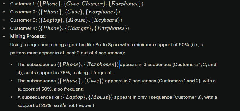
1. Data Marts
Definition of Data Marts
A data mart is a subset of a data warehouse designed to serve a specific business unit, department, or user group within an organization. It focuses on a particular subject area or business function (e.g., sales, marketing, finance) and contains a smaller, more focused dataset compared to a data warehouse. Data marts are typically created to provide faster access to data, improve query performance, and meet the specific analytical needs of a targeted group of users.
- Purpose: Data marts enable business users to perform targeted analytics, reporting, and decision-making without having to navigate the complexity of an entire data warehouse.
- Example: A retail company might have a data mart specifically for the sales department, containing only sales-related data like transactions, customer purchases, and product performance.
Types of Data Marts
Data marts can be classified into different types based on their structure, data source, and relationship with the data warehouse. The question specifically focuses on dependent vs. independent data marts, but I’ll also briefly mention another common type for completeness.
-
Dependent Data Marts
-
Definition: A dependent data mart is sourced directly from a centralized data warehouse. It relies on the data warehouse for its data, meaning the data is extracted, transformed, and loaded (ETL) from the data warehouse into the data mart.
-
Characteristics:
-
Data consistency is high because it inherits the cleansed, integrated data from the data warehouse.
-
It is part of a top-down approach, where the data warehouse is built first, and data marts are created as subsets for specific departments.
-
Changes in the data warehouse (e.g., schema updates) directly affect the dependent data mart.
-
-
Example: A company with a data warehouse containing all enterprise data (sales, HR, finance) creates a dependent data mart for the marketing team, pulling only marketing-related data (e.g., campaign performance, customer demographics) from the warehouse.
-
Advantage: Ensures consistency and reduces redundancy since data is managed centrally in the data warehouse.
-
Disadvantage: Dependency on the data warehouse can lead to delays if the warehouse is not updated or if there are bottlenecks in the ETL process.
-
-
Independent Data Marts
-
Definition: An independent data mart is created without relying on a centralized data warehouse. It sources data directly from operational systems, external sources, or other databases, and is built to serve a specific business unit independently.
-
Characteristics:
-
It follows a bottom-up approach, where the data mart is built first to meet immediate departmental needs, without waiting for a full data warehouse.
-
Data integration and consistency may be lower because it doesn’t benefit from the centralized cleansing and standardization of a data warehouse.
-
It operates independently, so changes in other systems don’t directly affect it.
-
-
Example: A finance department builds an independent data mart by pulling financial transaction data directly from the company’s operational database to analyze budgets and expenses, without using a data warehouse.
-
Advantage: Faster to implement since it doesn’t require a data warehouse, making it suitable for smaller organizations or urgent needs.
-
Disadvantage: Risk of data inconsistency (e.g., different data marts may have conflicting definitions of the same metric) and higher maintenance overhead if multiple independent data marts exist.
-
-
Hybrid Data Marts (for completeness, though not the focus):
-
Definition: A hybrid data mart combines data from both a data warehouse and other sources (e.g., operational systems or external data).
-
Characteristics: It balances the consistency of a dependent data mart with the flexibility of an independent one.
-
Example: A sales data mart might pull historical data from a data warehouse and real-time sales data directly from a transactional system.
-
Key Comparison (Dependent vs. Independent Data Marts):
-
Source of Data: Dependent data marts source data from a data warehouse, while independent data marts source data directly from operational systems or other sources.
-
Approach: Dependent data marts are part of a top-down approach (data warehouse first), while independent data marts follow a bottom-up approach (data mart first).
-
Consistency: Dependent data marts ensure higher data consistency due to centralized integration, whereas independent data marts may lead to inconsistencies across departments.
-
Implementation Time: Independent data marts are faster to set up since they don’t require a data warehouse, but dependent data marts may take longer due to their reliance on the warehouse.
-
Scalability: Dependent data marts scale better in large organizations with a centralized data warehouse, while independent data marts may lead to silos and redundancy in large setups.
Data Warehouse vs Operational Database
| Aspect | Data Warehouse | Operational Database |
|---|---|---|
| Purpose | Designed for analytical processing, reporting, and decision-making (OLAP). | Designed for transactional processing and day-to-day operations (OLTP). |
| Type of Data | Stores historical data for trend analysis, forecasting, and long-term insights. | Stores current, transactional data for real-time operations. |
| Granularity | Data is aggregated at a higher level (e.g., monthly sales summaries). | Data is detailed and granular (e.g., individual sales transactions). |
| Data Structure | Denormalized for faster query performance (e.g., star or snowflake schema). | Normalized to reduce redundancy and ensure data integrity. |
| Time Focus | Time-variant; includes historical data spanning years for analysis. | Time-invariant; focuses on current data with frequent updates. |
| Access Pattern | Read-heavy; optimized for complex queries and aggregations. | Read-write; optimized for quick inserts, updates, and deletes. |
| User Base | Used by analysts, data scientists, and executives for strategic decisions. | Used by operational staff for routine business processes (e.g., clerks). |
| Performance | Slower for updates but faster for analytical queries over large datasets. | Fast for transactional operations but slower for complex analytics. |
Characteristics of a Data Warehouse
A data warehouse has four defining characteristics:
-
Subject-Oriented:
- Focuses on specific business subjects or areas (e.g., sales, finance, inventory) rather than the entire organization’s operations.
- Example: A data warehouse might store all sales-related data for analysis, ignoring unrelated data like employee records.
-
Integrated:
- Combines data from multiple, heterogeneous sources (e.g., databases, flat files) into a consistent format.
- Example: Sales data from different regions with varying formats (e.g., dates as MM/DD/YYYY or DD-MM-YYYY) is standardized during integration.
-
Time-Variant:
- Stores historical data over extended periods to enable trend analysis and forecasting.
- Example: A data warehouse might keep sales data for the past 10 years, allowing users to analyze seasonal trends.
-
Non-Volatile:
- Data in a data warehouse is stable and not subject to frequent updates or deletes; it’s primarily used for read-only analysis.
- Example: Once sales data for a month is loaded, it isn’t modified, ensuring a consistent historical record for reporting.
Role of Dimensional Data and Granularity in Warehouse Design
Role of Dimensional Data in Warehouse Design
Definition of Dimensional Data:
Dimensional data refers to the structure used in a data warehouse to organize data for efficient querying and analysis, typically following a dimensional modeling approach (e.g., star schema or snowflake schema). It consists of two main types of tables:
- Fact Tables: Store quantitative data (metrics) that are analyzed, such as sales amounts, quantities sold, or revenue.
- Dimension Tables: Store descriptive attributes that provide context to the facts, such as time, product, customer, or location details.
Role in Warehouse Design:
-
Efficient Query Performance:
- Dimensional data organizes data into a structure that optimizes analytical queries (OLAP). For example, in a star schema, fact tables are linked to dimension tables, allowing users to quickly aggregate metrics (e.g., total sales) across dimensions (e.g., by region, by month).
- This structure reduces the need for complex joins compared to normalized operational databases, speeding up queries.
-
Simplified Data Analysis:
- Dimensions provide a way to "slice and dice" data, enabling users to analyze data from different perspectives. For instance, a sales fact table linked to a time dimension allows users to analyze sales trends by year, quarter, or month.
- This supports business intelligence tasks like reporting, forecasting, and decision-making.
-
Data Consistency and Integration:
- Dimension tables ensure consistency by standardizing descriptive data. For example, a product dimension table might unify product names and categories from multiple sources, ensuring all reports use the same definitions.
- This is critical in a data warehouse, which integrates data from heterogeneous sources (as per the "Integrated" characteristic of a data warehouse).
-
Support for Hierarchical Analysis:
- Dimensions often include hierarchies (e.g., a time dimension with levels like year → quarter → month → day), allowing users to drill down or roll up data for detailed or summarized analysis.
- Example: A user can analyze sales at the yearly level and then drill down to the monthly level to identify seasonal patterns.
Example:
In a retail data warehouse, a fact table might store daily sales amounts, linked to dimension tables for time (date, month, year), product (name, category), and store (location, region). This structure allows a manager to query "total sales of electronics in the West region for Q1 2024" efficiently.
Role of Granularity in Warehouse Design
Definition of Granularity:
Granularity refers to the level of detail at which data is stored in a data warehouse. It determines the smallest unit of data available for analysis (e.g., daily sales vs. monthly sales summaries).
- Fine Granularity: More detailed data (e.g., sales per transaction).
- Coarse Granularity: More aggregated data (e.g., sales per month).
Role in Warehouse Design:
-
Determines Analytical Flexibility:
-
The granularity level defines how detailed the analysis can be. Finer granularity (e.g., sales per transaction) allows for more detailed analysis, such as identifying patterns at the hourly or daily level.
-
However, coarser granularity (e.g., monthly sales) may suffice for high-level strategic reporting and reduces storage needs.
-
Example: If a warehouse stores sales data at the daily level, users can analyze daily trends, but if it only stores monthly aggregates, daily patterns cannot be studied.
-
-
Impacts Storage and Performance:
-
Finer granularity requires more storage space and can slow down query performance due to the larger volume of data. For instance, storing every sales transaction for a large retailer generates massive datasets.
-
Coarser granularity reduces storage needs and speeds up queries but limits the depth of analysis.
-
Warehouse designers must balance these trade-offs based on user needs. For example, a warehouse might store detailed data for recent years (e.g., last 2 years at the daily level) and aggregated data for older periods (e.g., monthly summaries for 5+ years).
-
-
Affects Data Loading and ETL Processes:
-
The granularity level influences the Extract, Transform, Load (ETL) process. Finer granularity requires more complex transformations to handle large volumes of raw data from operational systems, while coarser granularity involves pre-aggregation during ETL, reducing load times.
-
Example: If the warehouse stores sales at the daily level, the ETL process must aggregate transactional data from the operational database into daily totals.
-
-
Supports Decision-Making Requirements:
-
Granularity must align with business needs. For operational reporting, finer granularity might be necessary (e.g., daily inventory levels), while strategic planning might require coarser granularity (e.g., yearly sales trends).
-
Example: A marketing team analyzing the impact of a daily promotion needs transaction-level granularity, while an executive planning annual budgets might only need monthly or yearly summaries.
-
Example:
A data warehouse for a chain of stores might choose a granularity of daily sales per store to allow detailed analysis of daily performance. If the granularity were set to yearly sales, the warehouse couldn’t support queries about seasonal or monthly trends, limiting its utility.
Combined Impact on Warehouse Design
-
Dimensional data and granularity work together to shape the warehouse’s structure and usability. Dimensional data provides the framework for organizing data (via fact and dimension tables), while granularity determines the level of detail within that framework.
-
For instance, a star schema with a time dimension (year, quarter, month, day) is only as useful as its granularity allows. If the granularity is set to monthly sales, the day level in the time dimension becomes irrelevant for analysis.
Difference between Data Mart and Data Warehouse
| Aspect | Data Mart | Data Warehouse |
|---|---|---|
| Scope | Focused on a specific business unit or department (e.g., sales, marketing). | Enterprise-wide, covering all business areas (e.g., sales, finance, HR). |
| Size | Smaller in size, containing a subset of data for a specific purpose. | Larger, storing vast amounts of data from across the organization. |
| Data Source | Often sourced from a data warehouse (dependent) or directly from systems (independent). | Sourced from multiple operational systems, databases, and external sources. |
| Complexity | Simpler structure, designed for quick access and specific queries. | More complex, integrating heterogeneous data with a broader scope. |
| User Base | Used by a specific group or department (e.g., marketing team). | Used by the entire organization, including analysts and executives. |
| Implementation Time | Faster to implement due to its focused scope. | Takes longer to build due to its enterprise-wide scope and integration needs. |
| Data Integration | May have less integration (especially independent data marts). | Highly integrated, ensuring consistency across all data sources. |
| Cost | Lower cost due to smaller scale and simpler design. | Higher cost due to larger scale, complexity, and infrastructure requirements. |
OLAP vs OLTP
| Feature | OLTP (Online Transaction Processing) | OLAP (Online Analytical Processing) |
|---|---|---|
| Purpose | Day-to-day operations | Decision-making and analytics |
| Data Type | Highly detailed, real-time data | Summarized, historical data |
| Examples | Banking transactions, e-commerce checkout | Sales trends, customer segmentation |
| Operations | Insert, Update, Delete | Complex Queries, Aggregations |
| Storage Design | Normalized | Denormalized (Star/Snowflake schema) |
Difference between Database and Data Warehouse
OLTP Database
A database is designed to capture and record data from a variety of enterprise systems i.e. OLTP - Online Transaction Processing. OLTP includes resource planning, customer relationships, transaction management etc. OLTP database is an operational database which contains highly detailed live, real-time data.
These databases should operate consistently for the success of a business and there should be no error or ambiguity in the data that is being stored. The transactions stored in the OLTP databases are simple and direct which can be queried with speed and ease. However, databases work slowly for querying large amounts of data and can slowdown the transactional process which negatively affects the business.
OLAP Data Warehouse
On the other hand, data warehouses are designed to store summarized data from various databases or sources after transforming the data according to the business necessity for analysis, reporting and decision making, i.e. OLAP - Online Analytical Processing. Since data from various sources is stored in a warehouse, the structure of a warehouse should be thoroughly pre-planned.
Querying huge amounts of data is easy with data warehouses, and it does not generally affect business as fresh data is generally not dynamically stored in the data warehouse, rather data is updated periodically. Data stored is secure, reliable and can be easily managed and retrieved.
A simply analogy would be:
- OLTP: Cash register at a shop.
- OLAP: Monthly sales report for the shop’s owner.
Data Warehouses are built for OLAP.
Star Schema vs Snowflake Schema
(Covered in module 1 pdf in depth.)
ETL Process in Data Warehousing
Definition of ETL
ETL stands for Extract, Transform, Load, and it refers to the three-step process used to collect data from various sources, transform it into a suitable format, and load it into a data warehouse for analysis and reporting. This process is critical for ensuring that data in the warehouse is consistent, clean, and ready for analytical queries.
Steps of the ETL Process
-
Extract:
-
Purpose: This step involves retrieving raw data from multiple, often heterogeneous, source systems. These sources can include operational databases (e.g., transactional systems), flat files, APIs, external data feeds, or even legacy systems.
-
Activities:
- Identify and connect to data sources.
- Extract relevant data, which may be structured (e.g., SQL databases), semi-structured (e.g., JSON), or unstructured (e.g., text files).
- Handle issues like data access permissions, network latency, or source system downtime.
-
Example: Extracting sales data from a retail company’s transactional database, customer data from a CRM system, and inventory data from an ERP system.
-
-
Transform:
-
Purpose: This step involves cleaning, standardizing, and restructuring the extracted data to ensure it is consistent, accurate, and suitable for the data warehouse. Transformation aligns the data with the warehouse’s schema and business requirements.
-
Activities:
- Data Cleaning: Remove duplicates, correct errors (e.g., fix inconsistent date formats like MM/DD/YYYY vs. DD-MM-YYYY), and handle missing values (e.g., impute or flag missing data).
- Data Integration: Combine data from different sources by resolving inconsistencies (e.g., unifying customer IDs from different systems).
- Data Standardization: Convert data into a common format (e.g., standardizing currency to USD, converting weights to kilograms).
- Data Enrichment: Add derived attributes (e.g., calculating total sales from quantity and price).
- Data Aggregation (if needed): Pre-aggregate data to match the warehouse’s granularity (e.g., summing daily sales into monthly totals).
- Normalization/Denormalization: Adjust data to fit the warehouse schema (e.g., denormalizing data for a star schema).
-
Example: Transforming sales data by standardizing date formats, removing duplicate transactions, calculating total revenue per transaction, and mapping product IDs to a unified product dimension table.
-
-
Load:
- Purpose: This step involves loading the transformed data into the data warehouse, making it available for analysis and reporting.
- Activities:
- Load data into the appropriate tables (e.g., fact and dimension tables in a star or snowflake schema).
- Choose between full load (loading all data) or incremental load (loading only new/updated data since the last load).
- Ensure data integrity during loading (e.g., handling foreign key constraints).
- Optimize load performance to minimize downtime (e.g., using bulk loading techniques).
- Example: Loading the transformed sales data into a sales fact table and linking it to dimension tables (e.g., time, product, store) in the data warehouse.
Importance of ETL in Data Warehousing
- Data Consistency: ETL ensures that data from disparate sources is integrated and standardized, aligning with the "Integrated" characteristic of a data warehouse.
- Data Quality: The transformation step improves data quality by cleaning and validating data, ensuring accurate analysis.
- Support for Analysis: ETL prepares data for efficient querying by organizing it into a structure suitable for OLAP (e.g., star or snowflake schema).
- Historical Data Storage: ETL enables the loading of historical data, supporting the "Time-Variant" characteristic of a data warehouse.
Challenges in ETL
- Complexity: Handling large volumes of data from heterogeneous sources can be complex, especially during transformation.
- Performance: ETL processes can be time-consuming, particularly for large datasets, requiring optimization (e.g., parallel processing).
- Error Handling: Issues like missing data, inconsistent formats, or source system failures need to be managed to avoid loading incorrect data.
Module 2
Formal Definition of Association Rules (Support, Confidence, Frequent Itemsets).
Association Rules
An association rule is an implication of the form:
What is an implication btw?
It's a simple rule we studied back in automata theory which states that :
if {a} then {b}
or
It has two key metrics:
- Support — How frequently {A, B} occurs.
- Confidence — The probability of {B} given {A}.
Confidence = Support({A, B}) / Support({A})
And sometimes:
- Lift measures the strength compared to random chance.
Lift = Confidence / Support({B})
Antecedent and Consequent in Association Rules (Important)
In Association Rules, the terminology is inspired by logic:
- Antecedent (LHS): the "if" part of the rule — the condition.
- Consequent (RHS): the "then" part of the rule — the outcome.
💡 Example:
If you find a frequent itemset {Bread, Butter}, you can generate two rules:
- Bread ⇒ Butter
- Butter ⇒ Bread
Here:
-
For rule Bread ⇒ Butter:
Antecedent = {Bread}
Consequent = {Butter} -
For rule Butter ⇒ Bread:
Antecedent = {Butter}
Consequent = {Bread}
When computing confidence:
Confidence = Support(Itemset) / Support(Antecedent)
Rule: Bread ⇒ Butter
Support({Bread, Butter}) = 0.8
Support({Bread}) = 1.0
Confidence = 0.8 / 1.0 = 0.8
Significance of Lift and Correlation in Association Rule Mining
In Association Rule Mining, Support and Confidence are primary measures for evaluating the strength of a rule. However, they aren't always sufficient. This is where Lift and Correlation come in, providing deeper insights into the relationships between items.
Let's consider an association rule A⇒B (meaning "if A then B").
Lift measures how much more likely item B is to be purchased/occur when item A is purchased/occurs, compared to how often B is purchased/occurs independently of A.
The formula for Lift of rule A⇒B is:
Lift(A⇒B)=
Which can also be written as:
Lift(A⇒B) =
Where:
- P(A∪B) is the probability of both A and B occurring together (which is equivalent to the Support of the itemset {A,B}).
- P(A) is the probability of A occurring (Support of A).
- P(B) is the probability of B occurring (Support of B).
- P(B∣A) is the conditional probability of B given A (which is the Confidence of A⇒B).
Significance/Interpretation of Lift:
-
Lift = 1: This indicates that the occurrence of A has no effect on the occurrence of B. In other words, A and B are independent events. The rule A⇒B is not particularly interesting because B is just as likely to occur whether A is present or not.
-
Lift > 1: This is the most interesting scenario. It means that the occurrence of A increases the likelihood of the occurrence of B. There is a positive association between A and B. The higher the lift value, the stronger the positive association. For example, if Lift = 2, it means that purchasing A makes you twice as likely to purchase B compared to a random purchase of B.
-
Lift < 1: This indicates that the occurrence of A decreases the likelihood of the occurrence of B. There is a negative association between A and B. This could mean they are substitute products (e.g., buying skim milk reduces the chance of buying whole milk) or simply that their occurrences are inversely related. While less common to seek in typical "market basket analysis" for cross-selling, this can be valuable for understanding competing products or for negative association rules (e.g., "if you buy X, you are less likely to buy Y").
Why Lift is Important: Lift helps filter out spurious or misleading rules that might have high confidence simply because the consequent item (B) is very common in the dataset. A high confidence rule might seem strong, but if B is purchased by almost everyone anyway, then A appearing might not genuinely lift the probability of B's purchase. Lift tells you if the relationship is truly insightful beyond mere co-occurrence or popularity.
Correlation (as a measure in ARM)
In the context of association rule mining, "correlation" is often used broadly to refer to measures that assess statistical dependence, similar to what Lift does. However, there are also specific statistical correlation coefficients (like the Chi-squared statistic, or correlation coefficients like Pearson's or Jaccard for binary data) that can be applied.
Definition: Correlation measures the statistical dependence between two items. It tells you if the occurrence of one item is related to the occurrence of another, and in what direction (positive or negative).
While Lift is a specific measure, when people talk about "correlation" in ARM, they are often referring to the general concept of statistical dependence that Lift helps to quantify.
Significance/Interpretation of Correlation (General):
- Positive Correlation: Similar to Lift > 1, indicates that items tend to appear together more often than expected by chance.
- Negative Correlation: Similar to Lift < 1, indicates that items tend to appear together less often than expected by chance.
- Zero/No Correlation: Similar to Lift = 1, indicates statistical independence.
Why Correlation is Important: Like Lift, correlation measures help to identify truly interesting rules by accounting for the base frequencies of items. If a rule has high support and confidence, but low or zero correlation, it might not be a strong predictor or a valuable insight. For instance, "buying bread ⇒ buying milk" might have high support and confidence, but if almost everyone buys both bread and milk anyway (they are very common items), the rule might not be as "interesting" as one that shows a strong, unexpected relationship between less common items. Correlation helps to differentiate between items that co-occur merely by chance or popularity, and those that have a genuine connection.