Classification and Prediction in Data Mining -- DW & DM -- Module 2
Index
- Introduction to Classification and Prediction -- The basics
- Supervised vs Unsupervised Learning
- Cluster Analysis
- Types of Data in Cluster Analysis
- 1. K-Means Clustering
- 2. K-Medoids Clustering
- Hierarchical Clustering Methods
- Agglomerative Approach -- Bottom Up Approach
- Divisive Hierarchical Clustering -- Top Down Approach
- Classification and Prediction Decision Trees
- 1. ID3 Algorithm (Iterative Dichotomiser 3)
- CART (Classification and Regression Trees)
- Prediction (or Regression) using Clustering Algorithms
- Transactional Patterns
- 1. Apriori Algorithm -- Association Rule Mining
- 2. F-P Growth Algorithm -- Association rule mining
Introduction to Classification and Prediction -- The basics
What is Classification?
Classification is all about assigning labels to data based on patterns it has learned from existing data.
It’s like training your brain:
- If you see a four-legged furry animal that barks, you classify it as a dog.
- If it purrs, it’s a cat.
In Technical Terms:
Given an input, classification answers:
"Which category does this data belong to?"
Examples:
| Scenario | Classification Task |
|---|---|
| Email Filtering | Classify as Spam or Not Spam. |
| Medical Diagnosis | Predict if a tumor is Benign or Malignant. |
| Image Recognition | Classify images into Cat, Dog, Bird. |
| Credit Scoring | Good or Bad credit risk. |
How Classification Works:
- Training Phase:
A model learns from labeled data.
Example:
[Height, Weight] → [Label: Male or Female]
- Testing Phase:
Model is given new, unseen data to predict the label.
Popular Classification Algorithms:
| Algorithm | Idea |
|---|---|
| Decision Trees | Split data into branches based on rules. |
| Naive Bayes | Based on probability and Bayes' theorem. |
| k-Nearest Neighbors | Classifies by looking at closest neighbors. |
| Support Vector Machine (SVM) | Finds the best boundary (hyperplane) between classes. |
2. What is Prediction?
Prediction is about estimating a value for new data based on past patterns.
Unlike classification, the output isn’t a category — it’s usually a numeric value.
Examples:
| Scenario | Prediction Task |
|---|---|
| Stock Market | Predict future stock price. |
| Weather Forecasting | Predict tomorrow's temperature. |
| House Pricing | Predict the selling price of a house. |
Difference between Classification & Prediction:
| Feature | Classification | Prediction |
|---|---|---|
| Output Type | Category/Label (discrete) | Numeric Value (continuous) |
| Example | Spam or Not Spam | Predicting stock price |
Process for Both:
-
Data Collection
Gather historical data. -
Data Preprocessing
Clean, filter, normalize, and format. -
Model Building
Train with algorithms. -
Evaluation
Test the model using new data. -
Deployment
Apply to real-world data.
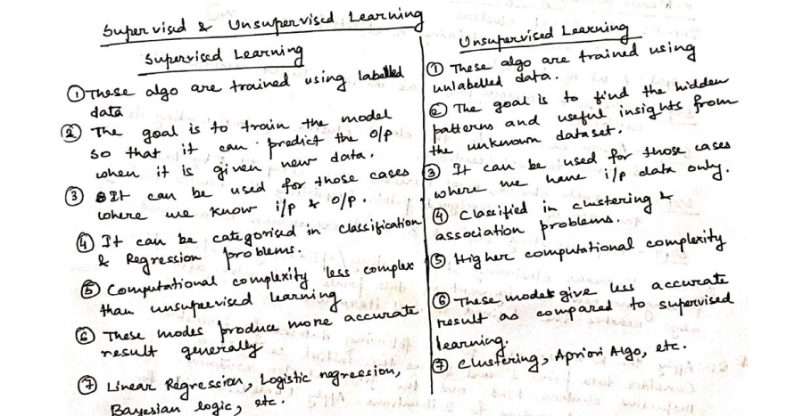
Supervised vs Unsupervised Learning
Cluster Analysis
What is a cluster?
Cluster is a group of objects that belongs to the same class. In other words, similar objects are grouped in one cluster and dissimilar objects are grouped in another cluster.
What is Clustering?
Clustering is the process of making a group of abstract objects into classes of similar objects, such that:
- Data points in the same cluster are similar to each other.
- Data points in different clusters are dissimilar.
Think of it as unsupervised learning — there are no labels like in classification.
For example, consider a dataset of vehicles given in which it contains information about different vehicles like cars, buses, bicycles, etc. As it is unsupervised learning there are no class labels like Cars, Bikes, etc for all the vehicles, all the data is combined and is not in a structured manner.
Now our task is to convert the unlabelled data to labelled data and it can be done using clusters.
The main idea of cluster analysis is that it would arrange all the data points by forming clusters like cars cluster which contains all the cars, bikes clusters which contains all the bikes, etc.
Simply it is the partitioning of similar objects which are applied to unlabelled data.
Simple Analogy:
Imagine you walk into a room full of people at a party.
Without knowing anyone’s names, you might group them like:
-
People standing near the snacks.
-
People deep in conversation.
-
People dancing.
That’s clustering!
You didn’t ask them who they were — you just used patterns (behavior/location).
Purpose of Clustering:
-
Identify natural groupings in data.
-
Simplify large datasets.
-
Spot outliers or unusual patterns.
-
Reveal hidden relationships.
Requirements of Clustering in Data Mining
The following points throw light on why clustering is required in data mining −
-
Scalability − We need highly scalable clustering algorithms to deal with large databases.
-
Ability to deal with different kinds of attributes − Algorithms should be capable to be applied on any kind of data such as interval-based (numerical) data, categorical, and binary data.
-
Discovery of clusters with attribute shape − The clustering algorithm should be capable of detecting clusters of arbitrary shape. They should not be bounded to only distance measures that tend to find spherical cluster of small sizes.
-
High dimensionality − The clustering algorithm should not only be able to handle low-dimensional data but also the high dimensional space.
-
Ability to deal with noisy data − Databases contain noisy, missing or erroneous data. Some algorithms are sensitive to such data and may lead to poor quality clusters.
-
Interpretability − The clustering results should be interpretable, comprehensible, and usable.
Common Clustering Algorithms:
| Algorithm | Idea | Use Case Example |
|---|---|---|
| K-Means | Divides data into K groups based on closeness. | Customer Segmentation in marketing. |
| Hierarchical Clustering | Builds a tree of clusters (dendrogram). | Gene expression analysis in biology. |
| DBSCAN | Clusters based on density rather than distance. | Detecting fraud or network attacks. |
Steps in Clustering:
-
Select Features
Choose which data points to group (e.g., income, age). -
Choose Similarity Measure
Usually distance-based:-
Euclidean Distance.
-
Manhattan Distance.
-
Cosine Similarity.
-
-
Run Algorithm
The algorithm assigns data points to clusters. -
Evaluate Quality
Visualize or measure:-
Intra-cluster similarity (tight groups).
-
Inter-cluster dissimilarity (clear separation).
-
Real-World Examples:
| Field | Use of Clustering |
|---|---|
| Marketing | Segmenting customers based on buying patterns. |
| Healthcare | Grouping patients by symptoms or treatment response. |
| Astronomy | Classifying stars or galaxies. |
| Social Networks | Detecting communities or friend groups. |
Example: K-Means Clustering (Basic Idea)
-
You specify
K(number of clusters). -
Algorithm randomly picks
Kcenters. -
Each point is assigned to the nearest center.
-
Centers are recalculated as the mean of assigned points.
-
Repeat until the clusters stabilize.
Types of Data in Cluster Analysis
Types Of Data Used In Cluster Analysis Are:
- Interval-Scaled variables
- Binary variables
- Nominal, Ordinal, and Ratio variables
- Variables of mixed types
1. Interval-Scaled variables
**Interval-scaled variables are continuous measurements of a roughly linear scale.
Typical examples include weight and height, latitude and longitude coordinates (e.g., when clustering houses), and weather temperature.
The measurement unit used can affect the clustering analysis. For example, changing measurement units from meters to inches for height, or from kilograms to pounds for weight, may lead to a very different clustering structure.
Why it matters:
Distance-based algorithms like K-Means work best here, since values have real physical meaning and mathematical operations make sense.
2. Binary variables
Definition:
A binary variable is a variable that can take only 2 values. Typically:
0 = Absence
1 = Presence
📏 Example:
-
Gender (
Male= 0,Female= 1) -
Has account:
Yes(1)/No(0)
💡 Similarity Measurement:
- Use Jaccard coefficient or Simple Matching depending on whether 0 and 1 are equally important.
3. Categorical (Nominal) Variables.
A generalization of the binary variable in that it can take more than 2 states, e.g., red, yellow, blue, green. Labels or names without inherent numerical meaning.
Example:
- Blood type:
A,B,AB,O - City names:
Delhi,Mumbai,Chennai - Product category:
Electronics,Furniture,Books
Similarity Measurement:
- Use Hamming distance or simple matching.
4. Ordinal Variables
Variables that have a rank/order, but the distance between ranks isn’t known or uniform.
An ordinal variable can be discrete or continuous.
Example:
- Customer satisfaction:
Poor,Average,Good,Excellent - Education level:
High School,Bachelor,Master,PhD
Handling:
You can convert them to numerical ranks, but treat them carefully to avoid distorting the meaning.
e.g. Poor = 1, Average = 2 ... but the "gap" between 1 and 2 isn’t always the same as between 2 and 3.
5. Ratio-Scaled Intervals
Like interval data, but ratios are meaningful and values have a natural zero (can be initialized to zero by default).
Example:
- Weight
- Age (in exact years)
- Length
- Distance
- Salary
Why important:
You can apply multiplication/division here.
A person earning $60K makes twice as much as someone earning $30K.
6. Mixed-Type Variables
👉 Definition:
Datasets that contain a mix of all the above types.
📏 Example:
| Age (Interval) | Gender (Binary) | Job Type (Categorical) | Rating (Ordinal) |
|---|---|---|---|
| 25 | Male (0) | Engineer | Good |
💡 Solution:
- Normalize the numeric data.
- Use specialized similarity measures like Gower’s Similarity Coefficient for mixed data types.
Why This Matters:
Different data types need different distance metrics:
| Data Type | Typical Similarity Measure |
|---|---|
| Interval/Ratio | Euclidean / Manhattan distance |
| Binary | Jaccard / Simple Matching |
| Categorical | Hamming distance / Matching coefficient |
| Ordinal | Spearman’s rank / Normalized distance |
Types of Partitioning/Clustering methods
https://www.scaler.com/topics/data-mining-tutorial/partitioning-methods-in-data-mining/
Overview
Partitioning methods split your dataset into a fixed number of clusters (k clusters, where k is defined before starting).
The goal is to:
- Assign each data point to one and only one cluster.
- Make clusters internally cohesive (data points are similar to each other) and externally isolated (different from other clusters).
1. K-Means Clustering
Basic Idea:
Divides n objects into k clusters, where each object belongs to the cluster with the nearest mean (called the centroid).
The K-Means algorithm begins by randomly assigning each data point to a cluster. It then iteratively refines the clusters' centroids until convergence. The refinement process involves calculating the mean of the data points assigned to each cluster and updating the cluster centroids' coordinates accordingly. The algorithm continues to iterate until convergence, meaning the cluster assignments no longer change. K-means clustering aims to minimize the sum of squared distances between each data point and its assigned cluster centroid.
Before we proceed further, let's understand about :
What is a Centroid?
A centroid is the geometric center of a cluster.
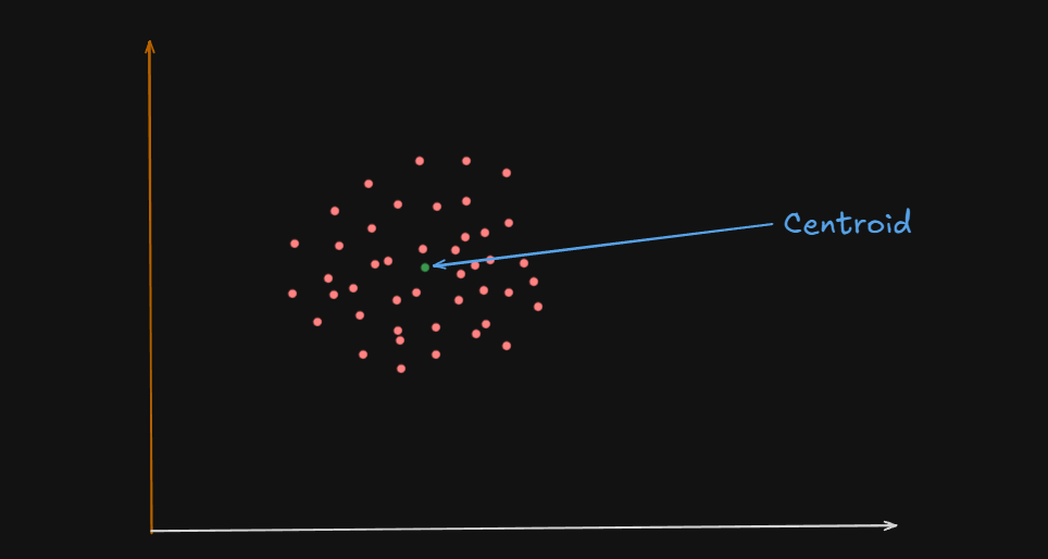
Or
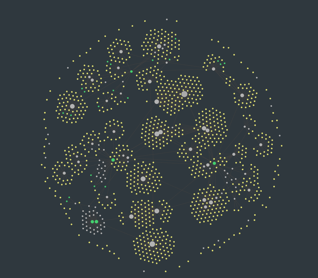
One could say that the centroid of these clusters are the big white circles at the center, and in some cases, the green circles
It’s like the average position of all the points (data samples) assigned to that cluster.
For example :
Let’s say you have a 2D space where each data point is represented by coordinates:
| Point | X | Y |
|---|---|---|
| A | 2 | 4 |
| B | 4 | 6 |
| C | 3 | 5 |
| If these three points belong to a single cluster, the centroid’s coordinates would be calculated like this: |
So the centroid of all these data points is
In higher dimensions(more number of variables), the centroid is still just the mean of each coordinate (feature) across all points in the cluster and the centroid formula scales as follows :
Why Is It Important?
1️⃣ The centroid acts like the "anchor" for a cluster. 2️⃣ During the K-Means algorithm:
- Data points are assigned to the cluster whose centroid is closest.
- Centroids are recalculated based on the new points assigned.
- This process continues until centroids stop changing.
Important:
- The centroid might not be an actual data point.
- It’s just the mathematical center, and sometimes no real data point is located there.
- In contrast, K-Medoids uses real data points as centers, not averages.
So, getting back to K-Means clustering,
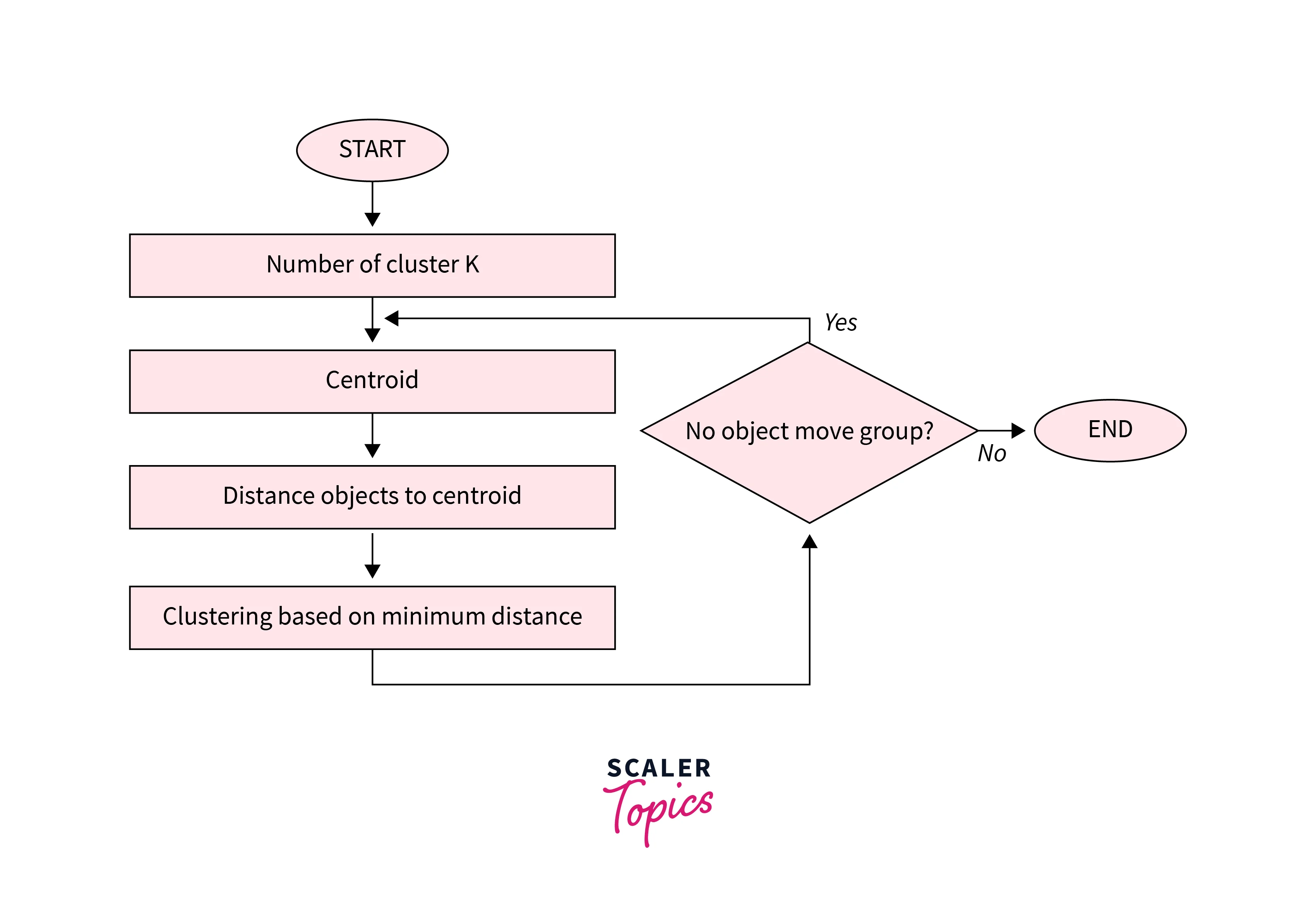
Algorithm of K-Means clustering
- Choose the number of clusters
k. - Randomly choose
kcentroids. - Assign each point to the nearest centroid. (This is done by calculating the distance of a point to all the centroids then assigning that point to the centroid with the lowest distance, thus creating a cluster)
- Re-compute centroids as the mean of all points in the cluster (using the centroid formula).
- Repeat steps 3 & 4 until centroids don’t change (convergence is reached) or a maximum number of iterations is reached.
Code
Here's a python program, if needed, to better understand K-Means algorithm
# K-Means partitioning


'''

Algorithm

1. Choose the number of clusters `k`.

2. Randomly choose `k` centroids.

3. Assign each point to the **nearest centroid**. (This is done by calculating the distance of a point to all the centroids then assigning that point to the centroid with the lowest distance, thus creating a cluster)

4. Re-compute centroids as the **mean** of all points in the cluster (using the centroid formula).

5. Repeat steps 3 & 4 until centroids don't change (convergence is reached) or a maximum number of iterations is reached.

'''


from typing import Tuple, List, Dict

from random import randint

from math import sqrt


data_points = [(2, 3), (4, 5), (6, 7)]


class K_Means():

    def __init__(self, k:int, points: list[tuple[int|float]], max_iter:int):

        self.points = points

        self.k = k

        self.centroids_list = []

        self.max_iter = max_iter

        self.still_running = False

        self.cluster = {}

        self.iteration = 0


    def choose_centroids(self) -> List[Tuple[float]]:

        centroids_list = []

        for i in range(self.k):

            centroids_list.append((randint(0, 9), randint(0,9)))

        self.centroids_list = centroids_list


        return centroids_list

    def euclidean_distance(self, c1: tuple, c2: tuple) -> int|float:

        return sqrt((c2[0]-c1[0])**2  + (c2[1] - c1[1])**2)  # root-over((x_2 - x_1)^2 + (y_2 - y_1)^2)


    def assign_point_to_centroid(self) -> Dict:


        if not self.centroids_list:

            self.choose_centroids()


        self.still_running = True


        for self.iteration in range(self.max_iter):

            cluster = {i: [] for i in range(self.k)} # populate the dict with {0: [], 1: []} and so on...

            self.cluster = cluster


            new_centroids = []


            # Convergence check


            if self.centroids_list == new_centroids:

                self.still_running = False

                break

            # Assign points to the nearest centroid

            for i in range(len(self.points)):

                distances = [self.euclidean_distance(self.points[i], centroid) for centroid in self.centroids_list] # calculate the distance from a point to all the centroids

                min_index = distances.index(min(distances)) # get the centroid with the smallest distance and it's index in the list.

                cluster[min_index].append(self.points[i])

                self.cluster = cluster


            # Recompute the centroids


            for j in range(self.k):

                points_in_cluster = cluster[j]

                if points_in_cluster: # if points are in cluster, then compute new centroids

                    new_centroid = self.compute_centroid_2D(points_in_cluster)

                    new_centroids.append(new_centroid)

                else:

                    # Keep previous centroid if cluster is empty

                    new_centroids.append(self.centroids_list[j])


            self.centroids_list = new_centroids


        return cluster


    def check(self) -> bool:

        return self.still_running


    def compute_centroid_2D(self, points: list[tuple[int|float]]) -> Tuple[float]:

        length = len(points) # for x or y axis the total number of points will be equal to the number of tuples present inside the list.


        x_values = 0

        y_values = 0


        for i in range(len(points)):

            x_values+=points[i][0]

            y_values+=points[i][1]


        centroid_x = (x_values/length)

        centroid_y = (y_values/length)

        return (centroid_x, centroid_y)


k_means = K_Means(3, data_points, 10)

k_means.choose_centroids()  # Set initial centroids

print(k_means.assign_point_to_centroid())
Output (is random every time the program is run):
{0: [(4, 5), (6, 7)], 1: [(2, 3)], 2: []}
Advantages of K-Means
Here are some advantages of the K-means clustering algorithm -
- Scalability - K-means is a scalable algorithm that can handle large datasets with high dimensionality. This is because it only requires calculating the distances between data points and their assigned cluster centroids.
- Speed - K-means is a relatively fast algorithm, making it suitable for real-time or near-real-time applications. It can handle datasets with millions of data points and converge to a solution in a few iterations.
- Simplicity - K-means is a simple algorithm to implement and understand. It only requires specifying the number of clusters and the initial centroids, and it iteratively refines the clusters' centroids until convergence.
- Interpretability - K-means provide interpretable results, as the clusters' centroids represent the centre points of the clusters. This makes it easy to interpret and understand the clustering results.
Disadvantages of K-Means
Here are some disadvantages of the K-means clustering algorithm -
- Curse of dimensionality - K-means is prone to the curse of dimensionality, which refers to the problem of high-dimensional data spaces. In high-dimensional spaces, the distance between any two data points becomes almost the same, making it difficult to differentiate between clusters.
- User-defined K - K-means requires the user to specify the number of clusters (K) beforehand. This can be challenging if the user does not have prior knowledge of the data or if the optimal number of clusters is unknown.
- Non-convex shape clusters - K-means assumes that the clusters are spherical, which means it cannot handle datasets with non-convex shape clusters. In such cases, other clustering algorithms, such as hierarchical clustering or DBSCAN, may be more suitable.
- Unable to handle noisy data - K-means are sensitive to noisy data or outliers, which can significantly affect the clustering results. Preprocessing techniques, such as outlier detection or noise reduction, may be required to address this issue.
2. K-Medoids Clustering
Similar to K-Means, but instead of using the mean as a center, it uses an actual data point (called a medoid) to represent the center.
Before, we proceed with that however,
What is a Medoid?
A medoid is the most centrally located actual data point within a cluster.
Unlike a centroid (which is often an average, and not always a real data point) —
a medoid is always one of the original, real points from your dataset.
Imagine you have a group of houses on a map, and you want to choose a meeting point for a neighborhood gathering:
- Centroid (K-Means) would give you the average of all coordinates — this could end up in the middle of a lake or someone’s rooftop!
- Medoid (K-Medoids) would pick one actual house from the group, the one that minimizes total travel distance for all neighbors.
How Is the Medoid Selected?
- For each data point in a cluster, calculate the total distance to all other points in the same cluster.
- Choose the point with the lowest total distance.
- That point becomes the medoid — the most centrally located representative of the cluster.
Why Use Medoids?
✅ Robust to Outliers:
Since medoids are real points, extreme outliers don’t "pull" the center like they do in K-Means.
✅ Flexible Distance Metrics:
You’re not limited to Euclidean distance — you can use Manhattan distance, cosine similarity, Hamming distance, etc.
Example
Let’s say you have this simple dataset of 2D points:
| Point | X | Y |
|---|---|---|
| A | 2 | 4 |
| B | 4 | 6 |
| C | 3 | 5 |
| D | 9 | 9 |
In K-Means, the centroid would be "pulled" toward D because it's an outlier.
But in K-Medoids, the algorithm would likely select B or C as the medoid, since it’s an actual point and minimizes total distance to others.
Before we proceed further :
What is an Outlier?
An outlier is a data point that is significantly different or far away from the rest of the data.
It’s like that one kid in a class who’s either way taller or way shorter than everyone else — they don’t fit the typical pattern of the group.
Example :
| Student | Age |
|---|---|
| A | 21 |
| B | 22 |
| C | 21 |
| D | 20 |
| E | 54 |
Here, 54 is clearly an outlier.
It doesn’t match the pattern of the other students, who are all around 20–22 years old.
How Outliers Pull the Centroid
When you calculate a centroid, you are averaging all the points.
If one point is way off (an outlier), it will shift the average toward itself.
Example :
Imagine all these points on a line
[1, 2, 2, 3, 3, 3, 30]
If you compute the average, (centroid) :
Now, in comparison to what the value would be if we didn't have
So, if we see the difference, just because of one outlier, the value of the centroid was much higher (pulled towards it).
However stuff like this doesn't happen with Medoids or K-Medoids since we select an actual data point.
General K-Medoids Process:
-
Initialization
Randomly selectkmedoids (real data points). -
Assignment Step
Assign each data point to the nearest medoid based on Euclidean (or another) distance. -
Update Step
For each cluster:- Test each point in the cluster.
- Calculate the total distance from that point to all other points in the cluster.
- Choose the point with the lowest total distance as the new medoid.
-
Convergence Check
Repeat steps 2 and 3 until:- The medoids no longer change.
- Or a max number of iterations is reached.
Code
Here's a python program if needed, to understand K-Medoids better
# K-Medoids


'''

Algorithm


1. Initialization

    Randomly select `k` _medoids (real data points).

2. Assignment Step

    Assign each data point to the nearest medoid based on Euclidean (or another) distance.

3. Update Step

    For each cluster:

    - Test each point in the cluster.

    - Calculate the total distance from that point to all other points in the cluster.

    - Choose the point with the lowest total distance as the **new medoid**.

4. Convergence Check

    Repeat steps 2 and 3 until:

    - The medoids no longer change.

    - Or a max number of iterations is reached.


We use medoids because unlike centroids, which are often pulled towards outliers (the farthest data point), this doesn't happen with medoids, which is an actual data point within the dataset

'''


import random

from math import sqrt


data_points = [(2, 3), (4, 5), (6, 7)]


class KMedoids:

    def __init__(self, k:int, points:list[tuple[int|float]], max_iter:int):

        self.k = k

        self.points = points

        self.max_iter = max_iter

        self.medoids = []

        self.cluster = {}

        self.iteration = 0


    def euclidean_distance(self, c1: tuple, c2: tuple) -> int|float:

        return sqrt((c2[0]-c1[0])**2  + (c2[1] - c1[1])**2)  # root-over((x_2 - x_1)^2 + (y_2 - y_1)^2)


    def initialize_medoids(self):

        self.medoids = random.sample(self.points, self.k)


    def assign_points(self):


        self.initialize_medoids()

        cluster = {i: [] for i in range(self.k)}


        for i in range(len(self.points)):

            distances = [self.euclidean_distance(self.points[i], medoid) for medoid in self.medoids]

            min_index = distances.index(min(distances))

            cluster[min_index].append(self.points[i])

            self.cluster = cluster


    def update_medoids(self) -> list[tuple[int|float]]:

        medoids = []


        for cluster_points in self.cluster.values():


            if cluster_points == []:  # skip empty clusters

                continue

            min_distance_sum = float('inf')

            best_medoid = None


            for candidate in cluster_points:

                total_distance = sum(self.euclidean_distance(candidate, other) for other in cluster_points)


                if total_distance < min_distance_sum:

                    min_distance_sum = total_distance

                    best_medoid = candidate


            medoids.append(best_medoid)


        return medoids


    def fit(self):

        for _ in range(self.max_iter):

            self.assign_points()

            new_medoids = self.update_medoids()

            if new_medoids == self.medoids:

                break

            self.medoids = new_medoids

            self.iteration += 1


k_medoids = KMedoids(3, data_points, 10)

k_medoids.assign_points()

k_medoids.fit()

print(k_medoids.cluster)
Output (is random every time the program is run):
{0: [(4, 5)], 1: [(6, 7)], 2: [(2, 3)]}
Difference Between K-Means & K-Medoids Clustering
Here is a comparison between K-Means and K-Medoids clustering algorithms in a tabular format.
| Factor | K-Means | K-Medoids |
| Objective | Minimizing the sum of squared distances between data points and their assigned cluster centroids. | Minimizing the sum of dissimilarities between data points and their assigned cluster medoids. |
| Cluster Center Metric | Use centroids, which are the arithmetic means of all data points in a cluster. | Use medoids, which are representative data points within each cluster that are most centrally located concerning all other data points in the cluster. |
| Robustness | Less robust to noise and outliers. | More robust to noise and outliers. |
| Computational Complexity | Faster and more efficient for large datasets. | Slower and less efficient for large datasets. |
| Cluster Shape | Assumes spherical clusters and is not suitable for non-convex clusters. | Can handle non-convex clusters. |
| Initialization | Requires initial centroids to be randomly selected. | Requires initial medoids to be randomly selected. |
| Applications | Suitable for applications such as customer segmentation, image segmentation, and anomaly detection. | Suitable for applications where robustness to noise and outliers is important, such as clustering DNA sequences or gene expression data. |
Hierarchical Clustering Methods
Hierarchical clustering builds a tree-like structure called a dendrogram to represent nested groupings of data points based on similarity.
Unlike K-Means or K-Medoids, you don’t need to predefine the number of clusters — the algorithm shows how the data groups together at all levels.
Two Types of Hierarchical Clustering Methods are
1️⃣ Agglomerative (Bottom-Up Approach)
This is the most common method.
- Start: Each data point is its own cluster.
- Step-by-Step:
- Find the two closest clusters and merge them.
- Repeat until all points belong to one single cluster.
- Result: A nested hierarchy of clusters, visualized as a dendrogram.
2️⃣ Divisive (Top-Down Approach)
Less common but useful for specific cases.
- Start: All data points are in one big cluster.
- Step-by-Step:
- Split the cluster into smaller and smaller groups.
- Keep dividing until every point is its own cluster.
- Result: Also visualized as a dendrogram, but built top-down.
How Do You Decide Which Clusters to Merge or Split?
This depends on distance measurement and linkage criteria.
Distance Measures (how you measure similarity):
- Euclidean distance (straight-line distance)
- Manhattan distance (grid-like path)
- Cosine similarity (angle-based)
Linkage Criteria (how you choose which clusters to merge):
| Method | Description |
|---|---|
| Single Linkage | Minimum distance between two points from different clusters. |
| Complete Linkage | Maximum distance between two points from different clusters. |
| Average Linkage | Average distance between all pairs from two clusters. |
| Ward’s Method | Minimizes the total variance within clusters. |
Dendrogram Example:
A dendrogram looks like an upside-down tree.
- The height of the branches represents the distance between merged clusters.
- You can "cut" the dendrogram at any height to choose the number of clusters.
Real-World Use Cases:
- Biology: Classifying species based on genetic similarity.
- Document Grouping: Grouping similar research papers.
- Customer Segmentation: When you don’t know how many types of customers exist in advance.
Summary Table:
| Feature | Agglomerative | Divisive |
|---|---|---|
| Start With | Each data point as a cluster | All data points in one cluster |
| Process | Merge closest pairs | Split into smaller groups |
| End With | One cluster | N clusters of single points |
| Common Usage | Very common | Less common |
Agglomerative Approach -- Bottom Up Approach
This is the most popular form of hierarchical clustering.
Algorithm
- Firstly convert the data points to their own clusters, each point is treated as a cluster itself, so the dataset now becomes a "cluster of clusters"
- Select a
kvalue. - Choose a linkage type (the linkage method is used to choose which clusters to merge)
- Take two clusters at a time from the list of clusters, use the linkage method to find two clusters which are closest to each other and then merge them into a single cluster.
- After merging, recalculate the distance between this newly formed cluster and the remaining clusters, merging more clusters based on their distances.
- Repeat this entire process till the total length of the "cluster of clusters" becomes less than the chosen
k
Example :
Input data set:
data_points = [(1, 1), (2, 2), (5, 5), (8, 8), (9, 9)]
Output, with different k-values and different linkage types
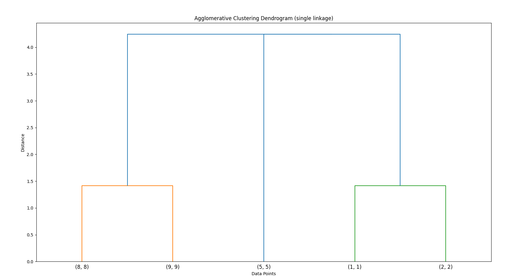
Using single linkage with k=2
(1, 1), (2, 2), (5, 5)], [(8, 8), (9, 9)
Using complete linkage with k=3
(1, 1), (2, 2)], [(5, 5)], [(8, 8), (9, 9)
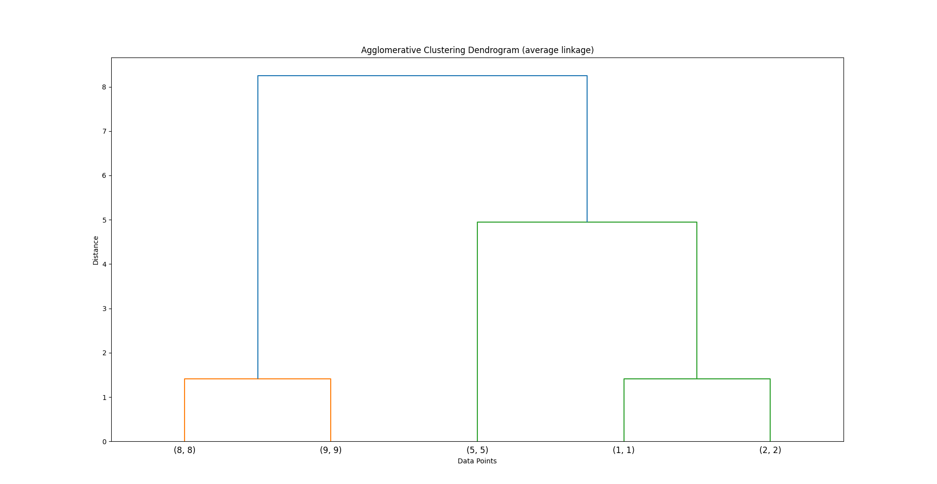
Using average linkage with k=4
(1, 1), (2, 2)], [(5, 5)], [(8, 8)], [(9, 9)
Note how the point (5,5) is considered close to the initial cluster [(1,1), (2,2)] with single linkage and k=2
How it becomes it's own cluster as a "mid-point cluster" at k=3 and complete linkage
And how it's considered too far from the first cluster, but considered close enough to the point (8,8) so it's clustered in with the 4'th point (8,8) at k=4 and average linkage
Why does this happen?
| Linkage Type | Behavior with bridge points like (5,5) |
|---|---|
| 🔗 Single Linkage | Looks for the closest pair. (5,5) gets attached early to whichever cluster has a point nearest to it — even if the rest of the cluster is far away. |
| 🔒 Complete Linkage | Looks for the farthest pair inside a merged cluster. If (5,5) would make the merged cluster's max distance too large, it avoids merging. |
| ⚖️ Average Linkage | Looks for the average distance to all points. If the cluster's center drifts too far from (5,5), it will hold off merging, even if one neighbor is close. |
And when k is set lower:
You’re forcing more compression, so borderline points like (5,5) get "absorbed" sooner — even if they might not be a perfect fit — just to reduce the cluster count.
When k is higher, there’s more freedom to hold off merging, so these points remain on their own longer.
Lastly, (optional):
Build a Dendrogram:
The process is visualized as a dendrogram — an inverted tree that shows the merging order and distances.
This is how it would be visualized as a dendrogram (for average linking)
Code
Here's a python program if needed to understand agglomerative clustering better
# Agglomerative clusters


'''

Algorithm


0. Firstly convert the data points to their own clusters, each point is treated as a cluster itself, so the dataset now becomes a "cluster of clusters"

1. Select a `k` value.

2. Choose a linkage type (the linkage method is used to choose which clusters to merge)

3. Take two clusters at a time from the list of clusters, use the linkage method to find two clusters which are closest to each other and then merge them into a single cluster.

4. After merging, recalculate the distance between this newly formed cluster and the remaining clusters, merging more clusters based on their distances.

5. Repeat this entire process till the total length of the "cluster of clusters" becomes less than the chosen `k`


'''


from math import sqrt


data_points = [(1, 1), (2, 2), (5, 5), (8, 8), (9, 9)] # Our data set


class AgglomerativeClustering():

    def __init__(self, points: list[tuple[int|float]], k: int, linkage_type="single linkage"):

        self.points = points

        self.k = k

        self.cluster = [[point] for point in points] # Converting each point into it's own clusters

        self.linkage_type = linkage_type

        print(f"Using {self.linkage_type} with k={self.k}")


    def euclidean_distance(self, c1: tuple, c2: tuple) -> int|float:

        return sqrt((c2[0]-c1[0])**2  + (c2[1] - c1[1])**2)  # root-over((x_2 - x_1)^2 + (y_2 - y_1)^2)


    # Single Linkage

    def closest_clusters_single_linkage(self, cluster1: list[tuple], cluster2: list[tuple]) -> float:

        return min(self.euclidean_distance(p1, p2) for p1 in cluster1 for p2 in cluster2)

    # complete linkage

    def closest_clusters_complete_linkage(self, cluster1: list[tuple], cluster2: list[tuple]) -> float:

        return max(self.euclidean_distance(p1, p2) for p1 in cluster1 for p2 in cluster2)

    # average linkage

    def closest_clusters_average_linkage(self, cluster1: list[tuple], cluster2: list[tuple]) -> float:

        distances = [self.euclidean_distance(p1, p2) for p1 in cluster1 for p2 in cluster2]

        return sum(distances)/ len(distances)


    def fit(self):

        while (len(self.cluster) > self.k):

            min_distance = float('inf') # min distance is reset to infinity in every search iteration

            to_merge = (None, None)


            # Find the pair of clusters which are closest to each other

            for i in range(len(self.cluster)):

                for j in range(i+1, len(self.cluster)):

                    if self.linkage_type == "single linkage": # default

                        dist = self.closest_clusters_single_linkage(self.cluster[i], self.cluster[j])

                    elif self.linkage_type == "complete linkage":

                        dist = self.closest_clusters_complete_linkage(self.cluster[i], self.cluster[j])

                    else: # average linkage

                        dist = self.closest_clusters_average_linkage(self.cluster[i], self.cluster[j])


                    if dist < min_distance:

                        min_distance = dist

                        to_merge = (i, j)


            # merge the two closest clusters

            i, j = to_merge

            if i < j:

                self.cluster[i].extend(self.cluster[j])

                del self.cluster[j]

            else:

                self.cluster[j].extend(self.cluster[i])

                del self.cluster[i]


agg_cluster_single = AgglomerativeClustering(data_points, 2)

agg_cluster_single.fit()

print(agg_cluster_single.cluster)


agg_cluster_complete= AgglomerativeClustering(data_points, 3, "complete linkage")

agg_cluster_complete.fit()

print(agg_cluster_complete.cluster)


agg_cluster_average = AgglomerativeClustering(data_points, 4, "average linkage")

agg_cluster_average.fit()

print(agg_cluster_average.cluster)
Strengths:
- No need to predefine the number of clusters.
- Easy to visualize with a dendrogram.
- Works well even when clusters are of different shapes and sizes.
Weaknesses:
- Computationally expensive (O(n²) or worse).
- Sensitive to noisy data and outliers.
- Once a decision is made to merge two clusters, it cannot be undone.
Divisive Hierarchical Clustering -- Top Down Approach
Process Step-By-Step:
We choose a k value.
We have a single cluster of all points.
For example:
[(1,1), (2,2), (5,5), (8,8), (9,9)]
and k=3
We compute the distances of all points to each other.
For example as I did in my code :
while len(new_super_cluster) + 1 < self.k:  # +1 because cluster still holds one group

            distances_dict = {}


            # Step 1: Compute pairwise distances

            for i in range(len(cluster)):

                for j in range(i + 1, len(cluster)):

                    distance = self.euclidean_distance(cluster[i], cluster[j])

                    distances_dict[(cluster[i], cluster[j])] = distance


            if not distances_dict:

                break  # nothing to split
We pick the two farthest points first and assign them to two separate clusters.
new_cluster1 = [(1,1)]
new_cluster2 = [(9,9)]
We remove these two points from the original cluster to remove confusion
Now we compute the distances of the remaining points to these two new clusters.
Now check each of the remaining points: (2,2), (5,5), (8,8).
(2,2)is closer to(1,1)→ goes tonew_cluster1.(5,5)is exactly in the middle but you can assign it to either (saynew_cluster1).(8,8)is closer to(9,9)→ goes tonew_cluster2.
Whichever point is closer to whichever cluster is assigned to that cluster.
Now we consider the cluster with the lesser number of elements as "done" and assign it to our final cluster list
If we want k=3 clusters, we still need to split further.
Usually the smaller cluster is considered “done.”
new_cluster2has fewer points:[(9,9), (8,8)].
So it is added to anew_super_cluster.
new_super_cluster = (9,9), (8,8)
cluster = [(1,1), (2,2), (5,5)] # remaining cluster which we need to work on further
Then we continue the process with the remaining cluster, pick farthest points, assign to two new clusters, remove them from the current cluster, compute distances to the remaining points in the cluster and then assign the one with the lesser number of elements to our final cluster list.
cluster = [(1,1), (2,2), (5,5)].
Farthest pair is (1,1) and (5,5).
Assign the remaining point (2,2):
- Distance to
(1,1)is smaller → goes tonew_cluster1.
new_cluster1 = [(1,1), (2,2)]
new_cluster2 = [(5,5)]
new_cluster2 has only 1 point, so it's smaller →
move [(5,5)] to new_super_cluster.
new_super_cluster = (9,9), (8,8)], [(5,5)
cluster = [(1,1), (2,2)]
cluster = [(1,1), (2,2)].
Farthest pair: (1,1) and (2,2).
Since these are the only two, they each become their own cluster.
And this process keeps on repeating till our original cluster's length becomes = our chosen k value since our condition is to keep running while the length of the cluster is greater than the chosen k, so the whole thing stops when our cluster length equals our chosen k.
So we get our final cluster as :
new_super_cluster = (9,9), (8,8)], [(5,5)], [(1,1)], [(2,2)
Outputs for different k-values
(1, 1), (2, 2)], [(5, 5), (8, 8), (9, 9) for k value: 2
(1, 1), (2, 2)], [(5, 5)], [(8, 8), (9, 9) for k value: 3
(1, 1), (2, 2)], [(5, 5)], [(9, 9)], [(8, 8) for k value: 4
- Build Dendrogram:
Like AHC, a dendrogram is formed — but this time it starts at the top and splits down.
Code
Here's a python program if needed to better understand divisive clustering
from typing import List

from math import sqrt


data_points = [(1, 1), (2, 2), (5, 5), (8, 8), (9, 9)] # Our data set


class DivisiveClustering():

    def __init__(self, points: list[tuple[int|float]], k: int):

        self.points = points

        self.k = k


    def euclidean_distance(self, c1: tuple, c2: tuple) -> int|float:

        return sqrt((c2[0]-c1[0])**2  + (c2[1] - c1[1])**2)  # root-over((x_2 - x_1)^2 + (y_2 - y_1)^2)


    def divisive_clustering(self) -> List:


        cluster = self.points.copy()  # start with all points as one cluster

        new_super_cluster = []


        while len(new_super_cluster) + 1 < self.k:  # +1 because cluster still holds one group

            distances_dict = {}


            # Step 1: Compute pairwise distances

            for i in range(len(cluster)):

                for j in range(i + 1, len(cluster)):

                    distance = self.euclidean_distance(cluster[i], cluster[j])

                    distances_dict[(cluster[i], cluster[j])] = distance


            if not distances_dict:

                break  # nothing to split


            # Step 2: Pick the two farthest points

            highest_distance = max(distances_dict.values())


            farthest_pair = [key for key, val in distances_dict.items() if val == highest_distance][0]


            point1, point2 = farthest_pair


            # Step 3: Assign points to the closest of the two

            new_cluster1 = []

            new_cluster2 = []


            for point in cluster:

                dist_to_1 = self.euclidean_distance(point, point1)

                dist_to_2 = self.euclidean_distance(point, point2)


                if dist_to_1 < dist_to_2:

                    new_cluster1.append(point)

                else:

                    new_cluster2.append(point)


            # Step 4: Choose one cluster to hold for future splits, the other goes to final list

            # Let's push the smaller one to the final list

            if len(new_cluster1) < len(new_cluster2):

                new_super_cluster.append(new_cluster1)

                cluster = new_cluster2

            else:

                new_super_cluster.append(new_cluster2)

                cluster = new_cluster1


        # Add the last remaining cluster

        new_super_cluster.append(cluster)


        return new_super_cluster


for k in [2, 3, 4]:

    div_cluster = DivisiveClustering(data_points, k)

    print(div_cluster.divisive_clustering(), f"for k value: {k}")
Strengths:
- Can be more accurate if the initial cluster is well-formed.
- Better for datasets where the global structure is more important than local relationships.
Weaknesses:
- Less common in practical use.
- Requires defining a clear splitting strategy, which can be subjective.
- Sensitive to the first split — a bad early split can ruin the final cluster arrangement.
Classification and Prediction : Decision Trees
What are Decision Trees?
They are tree-structured models used for:
- Classification (categorizing data),
- Regression (predicting numeric values),
- Rule Extraction (interpretable decision-making).
A decision tree splits data into branches based on feature values, asking questions at each node until it reaches a final decision at a leaf node.
So far all the algorithms we did, we have just done classification. Regression is something we haven't done yet.
Where are Decision Trees Used in Data Mining?
| Application Area | Purpose | Example |
|---|---|---|
| Classification | Predict categorical labels | Spam detection, disease diagnosis |
| Regression | Predict numerical values | Predict house prices, stock prices |
| Rule Mining / Knowledge Discovery | Extract human-readable patterns | Customer churn reasoning, fraud detection |
| Feature Selection | Identify most informative features | Preprocessing step in AI pipelines |
| Handling Missing Data | Splitting based on available info | Medical datasets, survey data |
| Ensemble Methods | Boosting or bagging models | Random Forest, Gradient Boosted Trees |
Common Decision Tree Algorithms in Data Mining
| Algorithm | Specialty |
|---|---|
| ID3 | Uses entropy and information gain for splitting. |
| C4.5 | Successor to ID3, handles continuous values, missing data. |
| CART | Classification and Regression Trees. Supports binary splits. |
| Random Forest | Ensemble of decision trees for better accuracy and generalization. |
Example: Simple Decision Tree Use Case
Imagine this dataset:
| Weather | Temperature | Play? |
|---|---|---|
| Sunny | Hot | No |
| Sunny | Cool | Yes |
| Overcast | Hot | Yes |
| Rainy | Cool | Yes |
A decision tree might split like:
Is Weather == Sunny?
 ├─ Yes → Is Temperature == Hot?
 │     ├─ Yes → Play: No
 │     └─ No  → Play: Yes
 └─ No → Play: Yes
1. ID3 Algorithm (Iterative Dichotomiser 3)
https://www.youtube.com/watch?v=mvveVcbHynE
https://www.youtube.com/watch?v=CWzpomtLqqs (ID3)
Invented by: Ross Quinlan (1986)
Use: Primarily for classification.
Goal: Build a decision tree by choosing attributes that give the most information gain at each split.
How it Works
Let's say we have this dataset:
| Outlook | Temperature | Humidity | Wind | Play Tennis |
|---|---|---|---|---|
| Sunny | Hot | High | Weak | No |
| Sunny | Hot | High | Strong | No |
| Overcast | Hot | High | Weak | Yes |
| Rain | Mild | High | Weak | Yes |
| Rain | Cool | Normal | Weak | Yes |
| Rain | Cool | Normal | Strong | No |
| Overcast | Cool | Normal | Strong | Yes |
| Sunny | Mild | High | Weak | No |
| Sunny | Cool | Normal | Weak | Yes |
| Rain | Mild | Normal | Weak | Yes |
| Sunny | Mild | Normal | Strong | Yes |
| Overcast | Mild | High | Strong | Yes |
| Overcast | Hot | Normal | Weak | Yes |
| Rain | Mild | High | Strong | No |
Step 1. Entropy Calculation
Entropy measures the disorder or impurity in your data.
This is the entropy calculation for the entire dataset
For a set
or
Where:
= probability of "Yes" = probability of "No"
Here, in total:
- 9 Yes
- 5 No
in the column of "Play Tennisi"
So,
Step 2: Calculate Information Gain for Each Attribute
For Outlook:
| Outlook | Temperature | Humidity | Wind | Play Tennis |
|---|---|---|---|---|
| Sunny | Hot | High | Weak | No |
| Sunny | Hot | High | Strong | No |
| Overcast | Hot | High | Weak | Yes |
| Rain | Mild | High | Weak | Yes |
| Rain | Cool | Normal | Weak | Yes |
| Rain | Cool | Normal | Strong | No |
| Overcast | Cool | Normal | Strong | Yes |
| Sunny | Mild | High | Weak | No |
| Sunny | Cool | Normal | Weak | Yes |
| Rain | Mild | Normal | Weak | Yes |
| Sunny | Mild | Normal | Strong | Yes |
| Overcast | Mild | High | Strong | Yes |
| Overcast | Hot | Normal | Weak | Yes |
| Rain | Mild | High | Strong | No |
Outlook has three values: Sunny, Overcast, Rain.
- Sunny: 5 samples → 2 Yes, 3 No.
- Overcast: 4 samples → 4 Yes.
- Rain: 5 samples → 3 Yes, 2 No.
Entropy for each:
Similarly :
Now, weighted entropy for outlook :
So :
Now, Information Gain of Outlook :
For Temperature
- Hot
4 samples 2 yes, 2 no - Mild
6 samples 4 yes, 2 no - Cool
4 samples 3 yes, 1 no
Since all the calculation by hand is quite time consuming, I will just write out the rest here :
For Humidity
- High: 7 samples , 3 yes, 4 no
- Normal: 7 samples, 6 yes, 1 no
For Wind
- Weak : 8 samples, 6 yes, 2 no
- Strong: 6 samples, 3 yes, 3 no
Creating the Decision Tree
✅ General Workflow for ID3:
- At the start: all attributes are candidates.
- At each split, after choosing an attribute, it is removed from consideration for that path.
- The remaining attributes are checked for Information Gain at each node until:
- Entropy is zero (pure class) (will be considered a Leaf Node)
- Attributes are exhausted (stop condition).
Now that we have all the data :
| Attribute | Information Gain |
|---|---|
| Outlook | 0.247 (Highest) |
| Humidity | 0.151 |
| Wind | 0.048 |
| Temperature | 0.029 |
We choose the root node with the highest information gain, in this case, outlook
            [ Outlook ]
           /     |     \
      Sunny  Overcast  Rain
Now for the Overcast Branch
Now we need to decide which node is a leaf node and which nodes will be continued.
We have the entropies of the three :
So Overcast is a leaf node.
Now, we will expand the remaining nodes
Sunny and Rain.
Before that, a quick note:
At every split, the dataset is reduced to a subset containing only the records that match the conditions so far. Information Gain is recalculated within this subset to decide the next best split.
Keeping that in mind,
For Sunny
We have the current subset as :
| Outlook | Temperature | Humidity | Wind | PlayTennis |
|---|---|---|---|---|
| Sunny | Hot | High | Weak | No |
| Sunny | Hot | High | Strong | No |
| Sunny | Mild | High | Weak | No |
| Sunny | Cool | Normal | Weak | Yes |
| Sunny | Mild | Normal | Strong | Yes |
So the highest gain in this table goes to Humidity.
Now for Outlook = Sunny and Humidity = High, we have PlayTennis = No and For Humidity = Normal, we have PlayTennis = Yes
These are pure splits, i.e the data is splitting into two outcomes purely.
                  [ Outlook ]
               /      |        \
          Sunny    Overcast    Rain
         /             |
Humidity              Yes
  /    |
High   Normal
|      |
No     Yes
So this becomes the current tree.
Similarly now for Rain, the subset becomes :
| Outlook | Temperature | Humidity | Wind | PlayTennis |
|---|---|---|---|---|
| Rain | Mild | High | Weak | Yes |
| Rain | Cool | Normal | Weak | Yes |
| Rain | Cool | Normal | Strong | No |
| Rain | Mild | Normal | Weak | Yes |
| Rain | Mild | High | Strong | No |
Now since we already split on Humidity before, the remaining unused attributes are Temperature and Wind, and since the next highest gain is on Wind:
So after Rain, we split on Wind
So the final decision tree becomes now :
                 [ Outlook ]
               /      |        \
          Sunny    Overcast    Rain
         /             |         |
Humidity              Yes       Wind
  /    |                         |  \
High   Normal                  Weak  Strong
 /     |                        |      \
No     Yes                     Yes      No
We stop the tree here since all attributes have been exhausted (Yes and No are the final outcomes so they are most certainly, leaf nodes).
CART (Classification and Regression Trees)
- Full form: Classification And Regression Trees
- Unlike ID3 (which only does classification), CART can handle:
- Classification (Yes/No, Class A/B/C).
- Regression (predicting continuous values like price, temperature, etc.).
https://www.youtube.com/watch?v=9K0M2KCyNYo
Difference between CART and ID3
| Feature | ID3 | CART |
|---|---|---|
| Splitting Metric | Information Gain (Entropy) | Gini Index |
| Output | Only Classification | Classification + Regression |
| Tree Structure | Multiway splits possible | Always Binary Splits (2 branches only) |
| Pruning | Post-pruning sometimes applied | Typically uses cost-complexity pruning |
Gini Index
In CART, the "purity" of a node is measured using Gini Impurity, not entropy.
The formula for Gini for a dataset
or :
Where:
is the probability of picking class at random. - Lower Gini = purer set.
⚡ CART Algorithm Steps:
-
For every attribute, and for every possible split point (yes, even numerical ones), compute the Gini Index of the split.
-
Choose the split (attribute + threshold) that gives the lowest Gini impurity in the two resulting nodes.
-
Repeat this process recursively for the child nodes.
-
Stop when:
- All records belong to the same class.
- There are no more attributes.
- The Gini index reaches 0.
-
Optionally: prune the tree to avoid overfitting.
Example
Let's work with a simplified dataset this time to save some time for us.
| Weather | PlayTennis |
|---|---|
| Sunny | No |
| Overcast | Yes |
| Rainy | Yes |
| Sunny | No |
| Sunny | Yes |
- For each attribute, compute the Gini impurity for possible splits.
- Choose the split that gives maximum reduction in impurity.
- Make binary splits only (unlike ID3 which might split multiway).
Why Binary Splits?
- Simplifies pruning.
- More predictable and balanced trees.
- Easier handling of numerical attributes (like age, income).
So let's start off by calculating the Gini Indexes of each attribute
Firstly, Gini Index of the entire table (Parent Node)
Total samples = 5
- Yes = 2
- No = 3
So,
Now, Gini Index of the Weather attribute
Weather has 3 subcategories:
- Sunny : 3 samples
2 No, 1 Yes - Overcast: 1 sample
Yes - Rainy: 1 sample
Yes
So,
Now, we need to calculate the weighted Gini index for the Weather attribute :
That's just :
So, $$Gini_{Weather} \ = \ (\frac{3}{5} \ \times \ 0.444) \ + \ (\frac{1}{5} \ \times 0) \ + (\frac{1}{5} \ \times 0)$$
Well since there are no more attributes in the table, let's proceed with creating the decision tree.
The tree will be split on Weather as it's the only attribute here
          [Weather]
         /    |     \
    Sunny  Overcast  Rainy
Now, for overcast and rainy both subsets have only one samples
| Weather | PlayTennis |
|---|---|
| Overcast | Yes |
| Rainy | Yes |
So both will have leaf nodes
          [Weather]
         /    |     \
    Sunny  Overcast  Rainy
      /       |        \
             Yes      Yes
As for the remaining node of Sunny,
| Weather | PlayTennis |
|---|---|
| Sunny | No |
| Sunny | No |
| Sunny | Yes |
This seems to be an impure split since the number of leaf nodes are not equally split.
In a traditional example we would have more attributes and more Gini Gains to decide for a split.
However since Weather is the only attribute present in the table, despite the rule of not using a used attribute again, we have no choice but to use Weather again for split.
As for what the leaf node will be, we do a majority voting and see that the value of No appears more than the value of Yes.
So the leaf node for Sunny will be No.
So we have our final decision tree as:
          [Weather]
         /    |     \
    Sunny  Overcast  Rainy
      /       |        \
    No       Yes      Yes
Note: In a real world example we would proceed with the calculation of the Gini Gains of all the attributes and then proceed like in the proceed of ID3, that is choosing the max Gini gain, using the corresponding attribute for a split in the tree, and then using the next unused attribute which has the highest gain among the remaining, just like how we did in ID3.
Since this example for learning purposes only, I saved the time taken by calculations by using a minimal dataset, something we would not see in most examples.
Example practice for CART
However for a sample practice example we can use this dataset
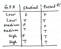
So we have the table as :
| GPA | Studied | Passed |
|---|---|---|
| Low | F | F |
| Low | T | T |
| Medium | F | F |
| Medium | T | T |
| High | F | T |
| High | T | T |
1. Gini index for the entire dataset
Total : 6
F: 2
T : 4
2. Gini Index for Studied attribute
Total samples of Studied = 6. Split between T and F
Studied = T
| GPA | Studied | Passed |
|---|---|---|
| Low | T | T |
| Medium | T | T |
| High | T | T |
Total: 3
T: 3
F: 0
Studied = F
| GPA | Studied | Passed |
|---|---|---|
| Low | F | F |
| Medium | F | F |
| High | F | T |
Total: 3
T: 1
F: 2
Weighted Gini:
3. Gini Index for GPA attribute
Now GPA has 3 values, we will split the dataset 3 times based on the values
Total GPA samples : 6
GPA = Low:
| Studied | Passed |
|---|---|
| F | F |
| T | T |
1 F, 1 T
GPA = Medium:
| Studied | Passed |
|---|---|
| F | F |
| T | T |
1 F, 1 T |
Same:
Gini = 0.5
GPA = High:
| Studied | Passed |
|---|---|
| F | T |
| T | T |
Both T: Gini = 0
Weighted Gini:
Choosing the best split
We have so far:
Studied: Gini = 0.2222GPA: Gini = 0.3333
Unlike what we do in ID3, where we choose the attribute with the highest information gain, in CART, we choose the attribute with the lowest Gini Index
So we will split on Studied
| GPA | Studied | Passed |
|---|---|---|
| Low | F | F |
| Low | T | T |
| Medium | F | F |
| Medium | T | T |
| High | F | T |
| High | T | T |
Since the T branch on Studied has the same output T, so it will become a leaf node (it's Gini was 0 as well)
However the F branch on Studied has two branching outputs 2 F and 1 T
So on the F branch of Studied we will split further on the next available attribute with the lowest Gini, that is, GPA.
Now for GPA
Low branch has the outputs : F = F and T = T, meaning not passed for Low GPA if the student didn't study, but passed for Low GPA is the student studied.
Medium branch has the same output.
High branch has the output T regardless of what Studied has, meaning the student will most definitely pass if they have a high GPA
So our tree will become
[Studied?]
 ├─ T: Passed = T
 └─ F:
       └─   GPA
          /  |   \
       Low Medium High
       /     |     /  \
     F|T    F|T   T    T
   (Tie)   (Tie) (Pure)(Pure)
Now we have a problem.
Both the Low and Medium branches of GPA have the same Gini Index as well, that creates a problem that we can't decide the split using the traditional way of deciding the minimum Gini Index.
So we need a tie-breaker.
Generally, other algorithms have tie-breakers in them such as random-picking, or alphabetical sorting or first occurrence.
In our case, to keep things simple we will use alphabetical sorting.
So if we sort F and T alphabetically, so the outputs for Low and Medium branches of GPA would be F.
This also makes sense if we think logically, that if a student did not study, and scored a Low GPA, they would most certainly not pass, and a Medium GPA generally gives a 50/50 chance of passing, hence our Gini Index of 0.5, but for tie-breaking purposes our decision tree will consider that as a F.
So our final decision tree becomes:
[Studied?]
 ├─ T: Passed = T
 └─ F:
       └─   GPA
          /  |   \
       Low Medium High
       /     |     /  \
     F       F    T    T
                (Pure)(Pure)
However this way of tie-breaking kind of ignores nuances, like there is a certain possibility of a person passing with a medium GPA if they didn't study. What about that? Or even in extreme cases, passing with a low GPA?
Well usually in such cases more better algorithms like random forest are used to grow multiple trees and use a majority voting metric to solve out the nuances or sometimes we can just modify the tree to return probabilities instead of hard values like:
| GPA | Passed Probability |
|---|---|
| Low | 40% Passed / 60% Failed |
| Medium | 50% Passed / 50% Failed |
| High | 90% Passed / 10% Failed |
This type of outputs can help a bit in dealing with such nuances.
Prediction (or Regression) using Clustering Algorithms
Before we proceed to pattern mining, let's take a step back and try to do some "prediction" or regression based on all the algorithms we studied so far.
Regression in Clustering-Based Models
Regression is the task of predicting a continuous value for a given input. In the context of clustering, regression can be approached by first grouping data points into clusters based on similarity, and then predicting a value for a new input based on the properties of the cluster it belongs to. This is a hybrid method that blends unsupervised learning (clustering) with supervised prediction (regression).
The common principle used in clustering-based regression is:
- Group similar data points into clusters.
- Assign a target value to each cluster, often as the average (mean) or representative value (like medoid) of the data points in that cluster.
- When a new data point is given, find the cluster it would most likely belong to.
- Predict the target value based on the cluster's assigned value.
Algorithms We Used for Clustering-Based Regression
1. Agglomerative Clustering Regression
Agglomerative clustering is a bottom-up approach where each data point starts in its own cluster, and pairs of clusters are merged as one moves up the hierarchy.
- Single Linkage: Merges clusters based on the minimum distance between their points.
- Complete Linkage: Uses the maximum distance between points in two clusters.
- Average Linkage: Uses the average pairwise distance between points in the two clusters.
How it handles regression:
- After clustering, each cluster's target is computed as the average of the values in that cluster.
- To predict a value for a new point, the algorithm finds the closest cluster based on the specified linkage rule.
Effect of changing k-values:
- More clusters (higher k) leads to finer groupings and more specific predictions.
- With smaller k, predictions are more general, potentially averaging over more diverse data.
Effect of linkage:
- Different linkage methods create different clustering structures.
- This leads to different predictions for the same input because the structure of the clusters and their centroids/medoids differ.
Example output
Using single linkage with k=2
Cluster:  ((1, 1), 10), ((2, 2), 20), ((5, 5), 15)], [((8, 8), 25), ((9, 9), 30)
Cluster targets:  {0: 15.0, 1: 27.5}
Prediction for (5, 10): 27.5


Using complete linkage with k=3
Cluster:  ((1, 1), 10), ((2, 2), 20)], [((5, 5), 15)], [((8, 8), 25), ((9, 9), 30)
Cluster targets:  {0: 15.0, 1: 15.0, 2: 27.5}
Prediction for (5, 10): 27.5


Using average linkage with k=4
Cluster:  ((1, 1), 10), ((2, 2), 20)], [((5, 5), 15)], [((8, 8), 25)], [((9, 9), 30)

Cluster targets:  {0: 15.0, 1: 15.0, 2: 25.0, 3: 30.0}
Prediction for (5,10): 25.0
As you can see, we have varying clusters based on k value and linkage choice.
✅ Pros: Flexible cluster shapes, more accurate in complex distributions.
⚠️ Cons: Slower, requires careful choice of k and linkage.
2. Divisive Clustering Regression
Divisive clustering is a top-down approach. It begins with all data points in one cluster and recursively splits them.
Splitting method used:
- At each step, the two most distant points are selected.
- All other points are assigned to the closer of the two.
- The smaller of the resulting clusters is considered finalized.
How it handles regression:
- Once clustering is complete, each cluster's target value is calculated as the average of the values in that cluster.
- For prediction, a new point is assigned to the cluster with the closest representative (often the medoid).
Effect of k-values:
- Higher k leads to smaller clusters, and predictions become more sensitive to local trends.
- Lower k merges more variance into single clusters, leading to more averaged-out predictions.
Medoid importance:
- Unlike agglomerative clustering (which may imply centroids), divisive clustering naturally leans toward medoid-based assignment for clearer distance-based decisions.
Example output
Cluster:  ((1, 1), 10), ((2, 2), 20)], [((5, 5), 15), ((8, 8), 25), ((9, 9), 30) for k value: 2
Cluster targets:  {0: 15.0, 1: 28.333333333333332} for k value: 2
Prediction for: (5, 10):  28.333333333333332, for k value: 2
Prediction for: (10, 10):  28.333333333333332, for k value: 2
Prediction for: (12, 12):  28.333333333333332, for k value: 2


Cluster:  ((1, 1), 10), ((2, 2), 20)], [((5, 5), 15)], [((8, 8), 25), ((9, 9), 30) for k value: 3
Cluster targets:  {0: 15.0, 1: 30.0, 2: 42.5} for k value: 3
Prediction for: (5, 10):  42.5, for k value: 3
Prediction for: (10, 10):  42.5, for k value: 3
Prediction for: (12, 12):  42.5, for k value: 3


Cluster:  ((1, 1), 10), ((2, 2), 20)], [((5, 5), 15)], [((9, 9), 30)], [((8, 8), 25) for k value: 4
Cluster targets:  {0: 15.0, 1: 30.0, 2: 60.0, 3: 85.0} for k value: 4
Prediction for: (5, 10):  85.0, for k value: 4
Prediction for: (10, 10):  60.0, for k value: 4
Prediction for: (12, 12):  60.0, for k value: 4
Why All Points Predict the Same in Lower k:
k = 2:
- You have only 2 clusters, so:
- One cluster holds the lower points
((1,1), (2,2)) - The other holds the rest, including higher-value targets like 25 and 30.
- One cluster holds the lower points
- All your new points (e.g.,
(5, 10),(10, 10),(12, 12)) are closer to that large high-value cluster. - ➤ So they all map to target ≈ 28.3
k = 3:
- One more cluster is formed — but the farthest points still stick together.
- So your new points still hit the cluster with
((8,8), (9,9)) - ➤ Hence, same prediction: 42.5
k = 4:
-
Now the clusters are more fine-tuned.
- For example,
((8,8), 25)and((9,9), 30)split into different clusters.
- For example,
-
So now,
(5,10)is closest to (8,8) → Predicts 85.0 -
(10,10)and(12,12)are closer to (9,9) → Predicts 60.0
3. K-Means
- Clustering basis: Minimizes within-cluster variance (Euclidean distance to centroids).
- Target Assignment: Each cluster target is the mean of all target values in that cluster.
- Prediction: New input is assigned to the closest centroid.
- Prediction not consistent: Due to the randomization involved in this algorithm, centroids are picked at random, so the clusters formed in each run of this algorithm are also random, leading to inconsistent predictions as you can see in the output below
Example output:
# For the same dataset

labeled_data = [((2, 3), 10), ((4, 5), 20), ((6, 7), 15), ((8, 9), 25), ((10, 11), 30)]


# Run 1

Centroids:  [(10.0, 11.0), (7.0, 8.0), (3.0, 4.0)]

Cluster:  {0: [((10, 11), 30)], 1: [((6, 7), 15), ((8, 9), 25)], 2: [((2, 3), 10), ((4,
5), 20)]}

Cluster targets:  {0: 30.0, 1: 20.0, 2: 15.0}

Prediction for (3, 4): 15.0

Prediction for (9, 10): 30.0

# Run 2

Centroids:  [(8.0, 9.0), (2.0, 3.0), (4.0, 5.0)]

Cluster:  {0: [((6, 7), 15), ((8, 9), 25), ((10, 11), 30)], 1: [((2, 3), 10)], 2: [((4,
5), 20)]}

Cluster targets:  {0: 23.333333333333332, 1: 10.0, 2: 20.0}

Prediction for (3, 4): 10.0

Prediction for (9, 10): 23.333333333333332

# Run 3

Centroids:  [(8.0, 9.0), (8, 5), (3.0, 4.0)]

Cluster:  {0: [((6, 7), 15), ((8, 9), 25), ((10, 11), 30)], 1: [], 2: [((2, 3), 10), ((4, 5), 20)]}

Cluster targets:  {0: 23.333333333333332, 1: None, 2: 15.0}

Prediction for (3, 4): 15.0

Prediction for (9, 10): 23.333333333333332

# Run 4

Centroids:  [(8.0, 9.0), (3.0, 4.0), (1, 8)]

Cluster:  {0: [((6, 7), 15), ((8, 9), 25), ((10, 11), 30)], 1: [((2, 3), 10), ((4, 5), 20)], 2: []}

Cluster targets:  {0: 23.333333333333332, 1: 15.0, 2: None}

Prediction for (3, 4): 15.0

Prediction for (9, 10): 23.333333333333332
As you can see, in some cases, different clusters were formed leading to different predictions for the same points across different runs.
4. K-Medoids
- Similar to K-Means, but uses medoids (real data points) instead of centroids.
- More robust to outliers since it avoids averaging extreme values.
✅ Pros: Higher accuracy than K-Means, more stable predictions.
⚠️ Cons: Slower than K-Means, especially with large datasets.
The problem of randomness affects K-Medoids as well during prediction, since medoids initially are picked randomly, so clusters are not the same in each run.
Example output
# For the same dataset

labeled_data = [((2, 3), 10), ((4, 5), 20), ((6, 7), 15), ((8, 9), 25), ((10, 11), 30)]


# Run 1

Medoids: [((2, 3), 10), ((8, 9), 25), ((6, 7), 15)]
Cluster Assignments: {0: [((2, 3), 10), ((4, 5), 20)], 1: [((8, 9), 25), ((10, 11), 30)], 2: [((6, 7), 15)]}
Cluster Target Values: {0: 15.0, 1: 27.5, 2: 15.0}
Prediction for (3, 4): 15.0
Prediction for (9, 10): 27.5


# Run 2

Medoids: [((4, 5), 20), ((8, 9), 25), ((10, 11), 30)]
Cluster Assignments: {0: [((2, 3), 10), ((4, 5), 20), ((6, 7), 15)], 1: [((8, 9), 25)],
2: [((10, 11), 30)]}
Cluster Target Values: {0: 15.0, 1: 25.0, 2: 30.0}
Prediction for (3, 4): 15.0
Prediction for (9, 10): 25.0


# Run 3

Medoids: [((2, 3), 10), ((8, 9), 25), ((4, 5), 20)]
Cluster Assignments: {0: [((2, 3), 10)], 1: [((8, 9), 25), ((10, 11), 30)], 2: [((4, 5), 20), ((6, 7), 15)]}
Cluster Target Values: {0: 10.0, 1: 27.5, 2: 17.5}
Prediction for (3, 4): 10.0
Prediction for (9, 10): 27.5

# Run 4

Medoids: [((10, 11), 30), ((2, 3), 10), ((6, 7), 15)]
Cluster Assignments: {0: [((10, 11), 30)], 1: [((2, 3), 10), ((4, 5), 20)], 2: [((6, 7), 15), ((8, 9), 25)]}
Cluster Target Values: {0: 30.0, 1: 15.0, 2: 20.0}
Prediction for (3, 4): 15.0
Prediction for (9, 10): 30.0
As you can see, in some cases, different clusters were formed leading to different predictions for the same points across different runs.
Takeaway from these example outputs :
- Higher k → More diverse predictions
- Medoid location (used internally for prediction) plays a huge role.
- Better clustering = better regression resolution.
- Careful choice of linkage algorithm (Agglomerative) = better cluster formation = more diverse prediction possibility.
- Partitioning algorithms are affected by randomness, leading to inconsistent predictions across different runs.
- As a result, hierarchical clustering perform better than partitioning algorithms on cluster formation and regression.
General Observations on Clustering-Based Regression
- Tradeoff between bias and variance: Fewer clusters mean more general predictions (high bias), while more clusters capture finer detail but may overfit (high variance).
- Choice of clustering algorithm affects prediction quality: Algorithms that better preserve natural groupings of data provide more accurate regression estimates.
- Choosing between centroid vs medoid: Centroids (means) can be misleading with outliers or non-convex distributions. Medoids (actual data points) are often more robust.
This approach is useful when explicit regression models are hard to define or when data shows natural groupings. It offers a way to incorporate the structure of the input space into predictions, making it valuable for complex or noisy datasets.
Transactional Patterns
Transactional data mining focuses on identifying patterns and relationships within datasets that represent transactions, such as sales, purchases, or website interactions. These patterns can be used for various purposes, like market basket analysis, fraud detection, and recommendation systems.
https://www.geeksforgeeks.org/frequent-pattern-mining-in-data-mining/
Key aspects of transactional data mining:
-
Frequent Pattern Mining:
This involves finding sets of items that frequently occur together in a transactional database.
-
Association Rule Mining:
This technique identifies rules that describe relationships between items in a dataset. For example, a rule might indicate that customers who buy bread and milk are likely to buy eggs.
For more on association, refer to module 1
-
Sequence Pattern Mining:
This focuses on identifying patterns that occur in a specific sequence over time, such as website click-streams or customer purchase sequences.
-
Data Preprocessing:
Data needs to be prepared before mining, including handling missing values, cleaning data, and transforming it into a suitable format.
Examples of transactional data mining applications:
-
Market Basket Analysis:
Identifying products that are frequently purchased together to optimize product placement, promotions, and inventory management.
-
Fraud Detection:
Analyzing transactional data to identify suspicious patterns that might indicate fraudulent activities, like credit card fraud or insurance fraud.
-
Recommendation Systems:
Suggesting products or services to customers based on their past purchase history or browsing behavior.
-
Customer Segmentation:
Grouping customers based on their purchasing habits to personalize marketing efforts and tailor product offerings.
Algorithms used in transactional data mining:
-
Apriori Algorithm:
A classic algorithm for finding frequent itemsets in transactional databases.
-
FP-Growth Algorithm:
Another popular algorithm for frequent pattern mining, known for its efficiency.
-
Other Algorithms:
Various other algorithms are used, including ECLAT, RARM, and ASPMS, each with its strengths and weaknesses.
Frequent Item sets
-
A frequent itemset is a set of items that occur together in a transactional dataset more often than a minimum support threshold.
-
Support= The proportion of transactions in which the itemset appears.
Example:
Transactions:
T1: {A, B, C}
T2: {A, B}
T3: {A, C}
T4: {B, C}
T5: {A, B, C}
If min_support = 0.6 (3 out of 5 transactions), then the frequent item sets would be:
{A} appears 4/5 → Frequent
{B} appears 4/5 → Frequent
{C} appears 4/5 → Frequent
{A, B} appears 3/5 → Frequent
{A, C} appears 3/5 → Frequent
{B, C} appears 3/5 → Frequent
{A, B, C} appears 2/5 → Not Frequent (below 0.6)
Closed Item sets
- A closed itemset is a frequent itemset that has no immediate superset with the same support.
- It tells you the most concise representation of frequent patterns.
Example (continued): If {A, B} and {A, B, C} have the same support, {A, B} is not closed — because {A, B, C} exists and has the same count.
If {A, B} has support 3, and {A, B, C} has support 2, {A, B} is closed.
Association Rules (important)
An association rule is an implication of the form:
What is an implication btw?
It's a simple rule we studied back in automata theory which states that :
if {a} then {b}
or
It has two key metrics:
- Support — How frequently {A, B} occurs.
- Confidence — The probability of {B} given {A}.
Confidence = Support({A, B}) / Support({A})
And sometimes:
- Lift measures the strength compared to random chance.
Lift = Confidence / Support({B})
Antecedent and Consequent in Association Rules (Important)
In Association Rules, the terminology is inspired by logic:
- Antecedent (LHS): the "if" part of the rule — the condition.
- Consequent (RHS): the "then" part of the rule — the outcome.
💡 Example:
If you find a frequent itemset {Bread, Butter}, you can generate two rules:
- Bread ⇒ Butter
- Butter ⇒ Bread
Here:
-
For rule Bread ⇒ Butter:
Antecedent = {Bread}
Consequent = {Butter} -
For rule Butter ⇒ Bread:
Antecedent = {Butter}
Consequent = {Bread}
When computing confidence:
Confidence = Support(Itemset) / Support(Antecedent)
Rule: Bread ⇒ Butter
Support({Bread, Butter}) = 0.8
Support({Bread}) = 1.0
Confidence = 0.8 / 1.0 = 0.8
Frequent Itemset Mining
- The process of finding all the itemsets that meet the minimum support in a dataset.
- This is the core job of algorithms like Apriori and FP-Growth.
- Once you get the itemsets, you can generate rules from them.
1. Apriori Algorithm -- Association Rule Mining
💡 What is Apriori?
The Apriori algorithm is a classic algorithm in data mining used for association rule learning.
Its purpose is to identify frequent itemsets in large transactional datasets and extract association rules — relationships that show how the occurrence of one item affects the occurrence of another.
🎯 Objective
- Discover sets of items (
itemsets) that frequently occur together. - Use these sets to generate rules that predict item presence based on other items in a transaction.
📚 Terminology
| Term | Meaning |
|---|---|
| Transaction | A single record/list of items bought together. |
| Itemset | A set of items (e.g., {Milk, Bread}). |
| Support | Fraction of transactions that contain the itemset. |
| Minimum Support | Threshold to consider an itemset as "frequent." |
| Confidence | Probability that consequent is present given antecedent. |
| Minimum Confidence | Threshold to consider a rule as valid. |
⚙️ Algorithm Overview
The Apriori algorithm follows this fundamental structure:
1️⃣ Generate Frequent Itemsets
- Scan the dataset to count individual items (1-itemsets).
- Remove items that don’t meet
minimum support. - Use the remaining items to generate candidate 2-itemsets.
- Scan the dataset again to count the frequency of these pairs.
- Remove itemsets that don’t meet
minimum support. - Repeat the process to generate
k-itemsetsuntil no more frequent itemsets can be found.
🧠 Apriori Principle:
If an itemset is frequent, all of its subsets must also be frequent.
If a subset is infrequent, any superset of it will be infrequent too.
2️⃣ Generate Association Rules
Once frequent itemsets are found:
-
For each frequent itemset:
-
Break it into antecedent → consequent pairs.
-
Compute Confidence:
-
-
Else, discard the rule.
Example
💼 Dataset:
| Transaction ID | Items |
|---|---|
| 1 | |
| 2 | |
| 3 | |
| 4 | |
| 5 |
🎯 Minimum Support: 0.6
(meaning itemsets must occur in at least 3 out of 5 transactions)
🧾 Step 1: 1-Itemsets
| Item | Count | Support |
|---|---|---|
| Milk | 3 | 0.6 |
| Bread | 5 | 1.0 |
| Butter | 4 | 0.8 |
All items meet the minimum support. Keep all.
🧾 Step 2: 2-Itemsets
Generate combinations from {Milk, Bread, Butter}:
| Itemset | Count | Support |
|---|---|---|
| 3 | 0.6 | |
| 2 | 0.4 ❌ | |
| 4 | 0.8 |
Only {Milk, Butter} is removed.
🧾 Step 3: 3-Itemsets
Generate combinations from surviving items:
| Itemset | Count | Support |
|---|---|---|
| 2 | 0.4 ❌ |
Doesn’t meet 0.6 support. Discard.
✅ Final Frequent Itemsets
{Milk}{Bread}{Butter}{Milk, Bread}{Bread, Butter}
🔁 Step 4: Generate Association Rules
Now check each itemset with 2 or more items:
For {Milk, Bread}:
Milk → Bread:✅ Bread → Milk:✅
For {Bread, Butter}:
Bread → Butter:✅ Butter → Bread:✅
🎉 Resulting Association Rules
| Rule | Confidence |
|---|---|
| Milk → Bread | 1.0 |
| Bread → Milk | 0.6 |
| Bread → Butter | 0.8 |
| Butter → Bread | 1.0 |
💡 Summary
- Apriori uses the downward closure property to prune unpromising candidates early.
- It incrementally builds larger item sets from smaller frequent ones.
- Association rules are formed based on the confidence metric.
- Simple, interpretable, but computationally heavy for very large datasets.
🧠 When to Use Apriori
- When datasets are small to medium.
- When rules should be transparent and easily explainable.
- When you can tolerate multiple dataset scans.
Code
For better understanding (how I did it), is to simply code the algorithm itself.
Here's a python program (if needed) for better understanding. Of course you need to have a good understanding of python before attempting to understand this.
import networkx as nx


# Transactions dataset


transactions = [

    ('Milk', 'Bread', 'Butter'),

    ('Bread', 'Butter'),

    ('Milk', 'Bread'),

    ('Milk', 'Bread', 'Butter'),

    ('Bread', 'Butter')

]


class Apriori():

    def __init__(self, data_set: list[tuple[str]], min_support: float):

        self.data_set = data_set

        self.min_support = min_support

        self.all_itemsets = []

        self.all_association_rules = []


    def get_frequent_itemsets(self):

        # will happen in levels


        self.support_dict1 = {} # dictionary of 1-itemsets having key-value pairs as item: support

        self.support_dict2 = {} # dictionary of 2-itemsets having key-value pairs as (item, item): support

        self.support_dict3 = {} # dictionary of 3-itemset having key-value pairs as (item, item, item): support


        self.set1 = {}

        self.set2 = {}

        self.set3 = {}


        itemsets = []

        for j in range(len(self.data_set)):

            # level 1: generate 1-itemsets.

            for k in range(len(self.data_set[j])):

                # get all the elements in each tuple and add to a set, preventing duplicates

                self.set1[self.data_set[j][k]] = None


        singleitemlist = list(self.set1.keys())

        item_count = 0


        # compute support for first itemset

        for i in range(len(singleitemlist)):

            for l in range(len(self.data_set)):

                if singleitemlist[i] in self.data_set[l]:

                    item_count+=1

            print(f"Count of {singleitemlist[i]} = {item_count}")


            support = item_count / len(self.data_set)


            # log the support in the dictionary for the items whose support are greater than or equals to min_support

            if support >= self.min_support:

                self.set1[singleitemlist[i]] = item_count

                self.support_dict1[singleitemlist[i]] = support

            else:

                # prune item from set1

                del self.set1[singleitemlist[i]]


            item_count=0 # reset the count for the next item to counted in the next iteration


        itemsets.append(self.set1.copy())


        item_count = 0 # reset item count to zero again to be reused later


        # level 2 - generate 2-itemsets based on the items which passed the support check in level 1


        for i in range(0, len(list(self.support_dict1.keys()))):

            for j in range(i+1, len(list(self.support_dict1.keys()))):

                self.set2[(list(self.support_dict1.keys())[i], list(self.support_dict1.keys())[j])] = None


        doubleitemlist = list(self.set2.keys())


        # compute support for the second itemset


        for i in range(0, len(doubleitemlist)):

            for l in range(0, len(self.data_set)):

                if (doubleitemlist[i][0] in self.data_set[l] and doubleitemlist[i][1] in self.data_set[l]): # get the occurence of the exact sequence of the 2-itemset in the original dataset

                    item_count+=1


            print(f"Count of {doubleitemlist[i]} = {item_count}")


            support = item_count / len(self.data_set)


            if (support >= self.min_support):

                self.set2[doubleitemlist[i]] = item_count

                self.support_dict2[doubleitemlist[i]] = support

            else:

                # prune from set2

                del self.set2[doubleitemlist[i]]


            item_count=0 # reset the count for the next item to counted in the next iteration


        itemsets.append(self.set2.copy())


        item_count = 0 # to be reused in level 3


        # level 3 - generate 3-itemset

        # feeling a bit lazy to code a DFS method to merge the tuples with a common element, so I will use networkx to solve this part.

        # Using networkx to generate a graph based on the list and then get the connected components as a list.

        # Found this at https://stackoverflow.com/a/62545221/16157201


        two_itemsetkeys_list = list(self.support_dict2.keys())

        graph = nx.Graph(two_itemsetkeys_list)

        tripleitemsetlist = list(map(tuple, nx.connected_components(graph))) # get the result back as a list of tuples


        # add to set3

        for i in range(0, len(tripleitemsetlist)):

                self.set3[tripleitemsetlist[i]] = None


        for i in range(0, len(tripleitemsetlist)):

            for l in range(0,  len(self.data_set)):

                if (tripleitemsetlist[i][0] in self.data_set[l] and tripleitemsetlist[i][1] in self.data_set[l] and tripleitemsetlist[i][2] in self.data_set[l]):

                    item_count+=1


            print(f"Count of {tripleitemsetlist[i]} = {item_count}")


            # compute support


            support = item_count / len(self.data_set)


            if (support >= self.min_support):

                self.set3[tripleitemsetlist[i]] = item_count

                self.support_dict3[tripleitemsetlist[i]] = support

            else:

                del self.set3[tripleitemsetlist[i]]


        itemsets.append(self.set3.copy())


        self.all_itemsets = itemsets


    def generate_association_rules(self):

        # will work with only itemsets of length >= 2


        rules = []

        to_delete = []

        confidence_list = []


        for support_dict in [self.support_dict2, self.support_dict3]:

            if (support_dict == {}):

                break # support dictionary is empty, doesn't have any item sets to generate association rules on

            keys_list = list(support_dict.keys())


            # get pairs of antecedents and consequents


            for i in range(0, len(keys_list)):

                for item in keys_list[i]:

                    antecedent = item


                    # compute confidence


                    confidence = support_dict.get(keys_list[i]) / self.support_dict1.get(antecedent)

                    print(f"Confidence for {keys_list[i]} with antecedent as {antecedent} = {confidence}")


                    confidence_list.append(confidence)


                if (all(x >= self.min_support for x in confidence_list)):

                    association_rule = {}

                    association_rule[keys_list[i]] = confidence_list[0]

                    association_rule[keys_list[i][::-1]] = confidence_list[1]

                    rules.append(association_rule)

                    confidence_list.clear()

                else:

                    to_delete.append(keys_list[i])

                    confidence_list.clear()

        for support_dict in [self.support_dict2, self.support_dict3]:

            if (support_dict == {}):

                break


            keys_list = list(support_dict.keys())


            for key in to_delete:

                if key in keys_list:

                    del support_dict[key] # prune the invalid association rule


        self.all_association_rules = rules


apriori = Apriori(transactions, 0.6)

apriori.get_frequent_itemsets()


print("All support dictionaries: ")

print(apriori.support_dict1)

print(apriori.support_dict2)

print(apriori.support_dict3)

print("\n")


print("All item sets: ")

print(apriori.all_itemsets)


print("\n")


apriori.generate_association_rules()

if (apriori.all_association_rules == []):

    print("No valid association rules found")

else:

    print("All association rules: ")

    assoc_rules = apriori.all_association_rules

    print(assoc_rules)
Output:
Count of Milk = 3
Count of Bread = 5
Count of Butter = 4
Count of ('Milk', 'Bread') = 3
Count of ('Milk', 'Butter') = 2
Count of ('Bread', 'Butter') = 4
Count of ('Bread', 'Milk', 'Butter') = 2
All support dictionaries:
{'Milk': 0.6, 'Bread': 1.0, 'Butter': 0.8}
{('Milk', 'Bread'): 0.6, ('Bread', 'Butter'): 0.8}
{}


All item sets:
[{'Milk': 3, 'Bread': 5, 'Butter': 4}, {('Milk', 'Bread'): 3, ('Bread', 'Butter'): 4}, {}]


Confidence for ('Milk', 'Bread') with antecedent as Milk = 1.0
Confidence for ('Milk', 'Bread') with antecedent as Bread = 0.6
Confidence for ('Bread', 'Butter') with antecedent as Bread = 0.8
Confidence for ('Bread', 'Butter') with antecedent as Butter = 1.0
All association rules:
[{('Milk', 'Bread'): 1.0, ('Bread', 'Milk'): 0.6}, {('Bread', 'Butter'): 0.8, ('Butter', 'Bread'): 1.0}]
Note that this code is for theoretical understanding purposes only, I haven't extended multi-item antecedent and consequent support or handling of k-frequent itemset generations
This output would indicate something like:
If a customer buys Milk, they are likely to also buy ('Bread',) (Confidence: 1.00)
If a customer buys Bread, they are likely to also buy ('Butter',) (Confidence: 0.80)
Why does this matter in business?
- Shops can arrange
BreadnearMilkbecause people who buy Milk tend to also buy Bread. - Discounts can be structured.
- Inventory planning.
- Cross-selling offers.
2. F-P Growth Algorithm -- Association rule mining
💡 What is F-P Growth?
The Frequent Pattern Growth (F-P Growth) algorithm is an advanced method for mining frequent itemsets without generating candidate sets like Apriori.
It uses a compressed structure called an FP-Tree (Frequent Pattern Tree) to store transactions, and extracts frequent patterns directly from it.
Why F-P Growth over Apriori?
| Apriori | F-P Growth |
|---|---|
| Generates candidates repeatedly. | No candidate generation. |
| Multiple full-dataset scans. | Usually 2 full-dataset scans only. |
| Memory-heavy for large datasets. | Uses compact FP-Tree for compression. |
| Slower with dense datasets. | Faster with both dense and sparse data. |
Algorithm Flow
1️⃣ Scan Dataset & Count Frequencies
- Go through the dataset once.
- Count the frequency of each item.
- Discard items below minimum support.
- Sort the surviving items in descending order of frequency.
2️⃣ Build the FP-Tree
- Initialize the root as
null. - For each transaction:
- Sort items according to global frequency.
- Insert items as a path into the tree.
- If part of the path already exists, increment the count at the node.
- Store links between nodes with the same item using a header table for fast access.
🪵 Example FP-Tree Build
Given transactions:
| TID | Items |
|---|---|
| 1 | |
| 2 | |
| 3 | |
| 4 | |
| 5 |
- Count frequencies:
Milk=3, Bread=5, Butter=4. - Minimum support = 0.6
Valid items: Milk, Bread, Butter. - Sort each transaction’s items by frequency:
Order: Bread > Butter > Milk.
Example insertion for T1 {Bread, Butter, Milk}:
Root
 └── Bread (1)
      └── Butter (1)
            └── Milk (1)
Further transactions add to this tree or extend new branches as needed.
3️⃣ Mine the FP-Tree (Recursive Extraction)
- For each item (lowest frequency first):
- Extract its conditional pattern base (prefix paths leading to the item).
- Build a conditional FP-Tree from this base.
- Recursively repeat the process on this new tree.
- Combine found patterns to produce all frequent itemsets.
Conditional Pattern Base Example
Let’s say for item Butter:
You gather paths like:
{Bread} : count 2
{Milk, Bread} : count 2
Final Output
A complete list of frequent itemsets that meet the minimum support threshold — just like Apriori, but found without brute-force combination testing.
Why is this Efficient?
- Compression: Repeated item combinations are stored in compact tree paths.
- No candidate generation: Saves computation time.
- Less scanning: Only 2 passes over the dataset.
- Recursive mining: Breaks down large problems into smaller ones via conditional trees.
When to Use F-P Growth?
- When the dataset is too large or dense for Apriori.
- When you need quick frequent pattern mining.
- When memory can handle tree-based storage.
Summary:
- Apriori is easy to understand and implement.
- F-P Growth is faster, cleaner, and smarter.
- Both aim to solve the same problem — mining frequent itemsets — but F-P Growth does it with structural optimization.
Code :
Here's a python program which covers F-P tree generation and frequent pattern mining in detail:
from typing import Dict

from itertools import combinations


# Transactions dataset


transactions = [

    ('Milk', 'Bread', 'Butter'),

    ('Bread', 'Butter'),

    ('Milk', 'Bread'),

    ('Milk', 'Bread', 'Butter'),

    ('Bread', 'Butter')

]


class Node:

    def __init__(self, name: str, count: int, parent):

        self.name = name

        self.count = count

        self.parent = parent

        self.child = None

        self.children = {}


class FPGrowth():

    def __init__(self, data_set: list[tuple[str]], min_support: float):

        self.data_set = data_set

        self.min_support = min_support

        self.tree_root = None


    def get_single_item_frequencies(self) -> Dict:

        singleitemset = {} # frequencies dictionary


        for i in range(len(self.data_set)):

            for j in range(len(self.data_set[i])):

                singleitemset[self.data_set[i][j]] = None  # add each item once as a key


        # count their frequencies now

        item_count = 0


        for i in range(0, len(list(singleitemset.keys()))):

            item = list(singleitemset.keys())[i]

            item_count = 0 # reset for every iteration

            for j in range(0, len(self.data_set)):

                for k in range(0, len(self.data_set[j])):

                    if (item == self.data_set[j][k]):

                        item_count+=1


            singleitemset[item] = item_count # update the frequency


        return singleitemset

    def filter_and_sort(self):


        frequency_dict = self.get_single_item_frequencies()


        self.support_dict1 = {} # single item support dictionary. No need to return this as we can just access it directly using self


        # filtration based on support


        to_delete = [] # keys which will be marked for pruning


        # calculate the support

        for i in range(0, len(list(frequency_dict.keys()))):

            item = list(frequency_dict.keys())[i]

            item_count = frequency_dict.get(item)


            support = item_count / len(self.data_set)


            if (support >= self.min_support):

                self.support_dict1[item] = support

            else:

                to_delete.append(item)

                # otherwise we just don't consider logging that item in support dict. Not pruning here since it's pointless and might end up affecting the transactions dataset.


        if (to_delete != []):

            for i in range(0, len(to_delete)):

                del self.support_dict1[to_delete[i]]

                del frequency_dict[to_delete[i]]


        print(self.support_dict1)


        # sorting the dict based on descending order of it's keys


        self.support_dict1 = dict(

            sorted(self.support_dict1.items(), key=lambda item: item[1], reverse=True)

        )


        self.frequency_dict = frequency_dict


    def build_fp_tree(self):

        transactions_list = self.data_set.copy()


        # reorder the elements within tuples within the list according to the order of the support dict


        new_transactions_list = []


        keys_list = list(self.support_dict1.keys())


        for tup in transactions_list:

            # create a new sublist

            item_list = [i for i in range(len(keys_list))] # prepopulate the sublist with the same number of elements as the number of keys in the support dict

            for item in tup:

                if (item in keys_list):

                    # get the index of this specific item within the keys list.

                    key_index = keys_list.index(item)

                    item_list[key_index] = item


            # now just check for any unwanted elements at any unwanted index.


            for item in item_list:

                if (type(item) == int):

                    idx = item_list.index(item)

                    del item_list[idx]


            # once all the items have been appended in the correct order, we append the item_list to the new_transactions_list


            new_transactions_list.append(item_list)


        print("Updated transactions list: ")

        print(new_transactions_list)

        print("\n")


        root = None # null node


        header_table = {}


        item_count = 0


        for i in range(len(new_transactions_list)):

            lst = new_transactions_list[i]

            for j in range (len(lst)):

                item = lst[j]

                item_count = 0 # reset the count

                if root is None:

                    # create the root node and add the first child node

                    root = Node("root", 0, None)

                    if item not in list(header_table.keys()):

                        item_count = 1

                        root.children[item] = Node(item, item_count, root)

                        root.child = root.children[item]

                        header_table[item] = item_count # log the occurrence in the header table

                else:

                    # root node has been created and first child node exists.

                    # get the list of children

                    children_list = list(root.children.keys())

                    # check if the current item is already a node or not

                    if item in children_list:

                        # increment the count of this child node by 1

                        count = header_table[item]

                        count+=1

                        header_table[item] = count

                        child = root.children[item]

                        child.count = count


                        # if this item is same as the direct child of the root node


                        if root.child.name == item:

                            root.child.count = count


                    else:

                        # item not present in header list, new node

                        item_count = 1

                        top = list(root.children.keys())[-1]

                        top_node = root.children[top]

                        root.children[item] = Node(item, item_count, top_node)

                        top_node.child = root.children[item]

                        header_table[item] = item_count


       # Add a None node at the very end of the tree, will be useful for traversal


        if root.children:

            last = Node("null", 0, root.children[list(root.children.keys())[-1]])

            root.children["END"] = last

            root.children[list(root.children.keys())[-1]].child = last


        self.header_table = header_table # make the header table globally accessible within the class now


        self.tree_root = root # make the tree globally accessible within the class now


    def print_tree(self):

        print(f"{self.tree_root.name} ({self.tree_root.count})")

        node = self.tree_root.child

        depth = 1


        while node is not None and node.name != "null":

            print("  " * (depth - 1) + f"↳ {node.name} ({node.count})")

            node = node.child

            depth += 1


    def find_patterns(self) -> Dict:

        patterns_dict = {}

        header_table = self.header_table.copy()


        while len(header_table) > 0:

            # Find item with minimum count

            min_val = min(header_table.values())

            end_node_name = [key for key, val in header_table.items() if val == min_val][0]


            # Traverse the path

            node = self.tree_root.child

            prefix_path = []


            while node is not None and node.name != "null":

                if node.name == end_node_name:

                    break

                prefix_path.append(node.name)

                node = node.child


            # Generate all pattern combinations including the end_node_name

            full_pattern = prefix_path + [end_node_name]

            for i in range(1, len(full_pattern)+1):

                for combo in combinations(full_pattern, i):

                    patterns_dict[frozenset(combo)] = min_val


            # Remove from header_table to process the next

            del header_table[end_node_name]


        return patterns_dict


    def filter_patterns_by_support(self, patterns_dict):

        return {pattern: count for pattern, count in patterns_dict.items() if count >= self.min_support}


fp_growth = FPGrowth(transactions, 0.6)


print(fp_growth.get_single_item_frequencies(), "\n")


fp_growth.filter_and_sort()

print(fp_growth.support_dict1, "\n")

fp_growth.build_fp_tree()


print("Header table: \n", fp_growth.header_table, "\n\n")


fp_growth.print_tree()

print("\n \n")


patterns = fp_growth.find_patterns()

frequent_patterns = fp_growth.filter_patterns_by_support(patterns)


print("Frequent Patterns:")

for pattern, count in frequent_patterns.items():

    print(set(pattern), "=>", count)
Output:
{'Milk': 3, 'Bread': 5, 'Butter': 4}

{'Milk': 0.6, 'Bread': 1.0, 'Butter': 0.8}
{'Bread': 1.0, 'Butter': 0.8, 'Milk': 0.6}

Updated transactions list:
'Bread', 'Butter', 'Milk'], ['Bread', 'Butter'], ['Bread', 'Milk'], ['Bread', 'Butter', 'Milk'], ['Bread', 'Butter'


Header table:
 {'Bread': 5, 'Butter': 4, 'Milk': 3}


root (0)
↳ Bread (5)
  ↳ Butter (4)
    ↳ Milk (3)


Frequent Patterns:
{'Bread'} => 5
{'Butter'} => 4
{'Milk'} => 3
{'Bread', 'Butter'} => 4
{'Bread', 'Milk'} => 3
{'Milk', 'Butter'} => 3
{'Bread', 'Milk', 'Butter'} => 3
Temporal Frequent Patterns
In real-world datasets, patterns don’t just exist in a static basket. They often change over time or occur in sequences. Here are some of the most interesting types:
1️⃣ Sequential Patterns
-
Focus: Order matters.
-
Example:
A customer buysMilk → Bread → Butteracross different visits, not in one basket. -
Algorithms:
- AprioriAll
- GSP (Generalized Sequential Pattern)
- PrefixSpan
2️⃣ Episode Patterns
- Focus: Events occurring close together in time windows.
- Example:
In a server log:
[Login Fail] → [Brute Force Detected] → [Firewall Alert]
— these happen within a 5-minute window often, but not necessarily in exact order.
3️⃣ Time-Decay Frequent Patterns
-
Focus: Recent patterns weigh more than old ones.
-
Example:
A store might give more weight to recent buying behavior to detect trends rather than treating old and new sales equally.
4️⃣ Periodicity Mining
-
Focus: Patterns that repeat at regular intervals.
-
Example:
A user might always order pizza on Fridays or there are server downtimes every night at 2 AM.
5️⃣ Temporal Association Rules
- Extends classic association rules with timestamps.
- Example:
IF {Bread} is bought on Monday → THEN {Butter} is bought within 2 days (confidence 0.8)
6️⃣ Spatio-Temporal Patterns
- Focus: Location + Time combined.
- Example:
People at [Location: Gym] → buy [Item: Protein Shake] within 10 minutes.
🔥 Summary Table
| Pattern Type | Use-case | Common Algorithm |
|---|---|---|
| Sequential Patterns | Web clickstreams, purchase sequences | PrefixSpan, SPADE |
| Episode Patterns | Event logs, anomaly detection | WINEPI, MINEPI |
| Time-Decay Frequent Patterns | Trending topics, hot products | Stream Mining |
| Periodicity Mining | Predictable habits / maintenance cycles | TSP, WARP |
| Temporal Association Rules | Time-based "if-then" patterns | T-Apriori |
| Spatio-Temporal Patterns | Mobility and behavior based on location & time | STPM, ST-Miner |