DBMS Numericals Practice
Identifying relationships between tables.
Example 1
Table A: Students
| StudentID | Name | |
|---|---|---|
| 1 | Alice | alice@example.com |
| 2 | Bob | bob@example.com |
| 3 | Charlie | charlie@example.com |
Table B: Student_ID_Cards
| CardID | StudentID | IssueDate | ExpiryDate |
|---|---|---|---|
| 101 | 1 | 2024-01-01 | 2028-01-01 |
| 102 | 2 | 2024-02-15 | 2028-02-15 |
| 103 | 3 | 2024-03-10 | 2028-03-10 |
1:1 relationship
Relationship table:
| StudentID | CardID |
|---|---|
| 1 | 101 |
| 2 | 102 |
| 3 | 103 |
| StudentID | Name | CardID | |
|---|---|---|---|
| 1 | Alice | alice@example.com | 101 |
| 2 | Bob | bob@example.com | 102 |
| 3 | Charlie | charlie@example.com | 103 |
Example 2
Table A: Authors
| AuthorID | Name |
|---|---|
| A1 | Jane Doe |
| A2 | John Smith |
| A3 | Amy Lin |
Table B: Books
| BookID | Title | AuthorID |
|---|---|---|
| B1 | Learning SQL | A1 |
| B2 | Advanced Databases | A1 |
| B3 | Distributed Systems | A2 |
| B4 | Data Structures in C++ | A3 |
| B5 | Data Science 101 | A1 |
1:N relationship
| AuthorID | BookID |
|---|---|
| A1 | B1 |
| A1 | B2 |
| A2 | B3 |
| A3 | B4 |
| A1 | B5 |
Merged table:
| BookID | Title | AuthorID |
|---|---|---|
| B1 | Learning SQL | A1 |
| B2 | Advanced Databases | A1 |
| B3 | Distributed Systems | A2 |
| B4 | Data Structures in C++ | A3 |
| B5 | Data Science 101 | A1 |
Example 3 – Many-to-Many Relationship
Table A: Students
| StudentID | Name |
|---|---|
| S1 | Alice |
| S2 | Bob |
| S3 | Charlie |
Table B: Courses
| CourseID | CourseName |
|---|---|
| C101 | Database Systems |
| C102 | Operating Systems |
| C103 | Artificial Intelligence |
N:N relationship since a single student can be enrolled in multiple courses, or multiple students can be enrolled in the same course, or multiple students can be enrolled in multiple courses
A potential relationship table would be:
| StudentID | CourseID |
|---|---|
| S1 | C101 |
| S2 | C101 |
| S2 | C102 |
| S3 | C101 |
| S3 | C103 |
Since this is a complex N:N relationship with multiple possible relationship tables, it's not possible to merge the two tables and reduce them into a single merged table.
Example 4 – Mixed Relationships
Table A: Teachers
| TeacherID | Name | Department |
|---|---|---|
| T1 | Dr. Sharma | Computer Sci. |
| T2 | Ms. Verma | Information Tech |
| T3 | Mr. Rao | Electronics |
Table B: Courses
| CourseID | CourseName | TeacherID |
|---|---|---|
| C101 | Database Systems | T1 |
| C102 | Operating Systems | T2 |
| C103 | Digital Electronics | T3 |
| C104 | Artificial Intelligence | T1 |
Table C: Students
| StudentID | Name | CourseID |
|---|---|---|
| S1 | Alice | C101 |
| S2 | Bob | C102 |
| S3 | Charlie | C101 |
Additional Info:
- A teacher can teach multiple courses, but each course is taught by only one teacher.
- Students can enroll in multiple courses, and each course can have many students.
First of all primary keys:
Table A: TeacherID
Table B: CourseID
Table C: StudentID
Now, since each course can only have one teacher, but a teacher can teach multiple courses, have a 1:N relationship for Teacher:Course
We can get a relationship table between tables A and B as :
| TeacherID | CourseID |
|---|---|
| T1 | C101 |
| T2 | C102 |
| T3 | C103 |
| T1 | C104 |
So can these two tables be merged? Yes, using the "many" table as the base, we already have a reduced table as Table B itself:
| CourseID | CourseName | TeacherID |
|---|---|---|
| C101 | Database Systems | T1 |
| C102 | Operating Systems | T2 |
| C103 | Digital Electronics | T3 |
| C104 | Artificial Intelligence | T1 |
Now, for tables B and C:
Since Students can enroll in multiple courses, and each course can have many students,
We have a N:N relationship for Student:Course.
A possible relationship table for these two would be:
| StudentID | CourseID |
|---|---|
| S1 | C101 |
| S2 | C101 |
| S2 | C102 |
| S3 | C101 |
| S3 | C103 |
And since there are way too many possibilities, we can't merge or reduce these two tables together.
Now, due to the fact that Table A is related to Table B and Table B is related to Table C, using a transitive dependency we can derive this relation:
"Teachers can teach multiple courses, and each course can have multiple students"
So
                - S1
               /
              /
		 - C101 -- S2
		  /    \
		 /      \
		/        - S3
       /
Teacher -- C102
      \
       \
        \
         - C103
So a single teacher can teach multiple students, i.e, a 1:N relationship between Table A and Table C
A potential relationship table could be:
| TeacherID | StudentID |
|---|---|
| T1 | S1 |
| T2 | S2 |
| T3 | S2 |
| T1 | S3 |
| T1 | S2 |
| T2 | S3 |
| T3 | S1 |
Can these two tables be merged?
Yes, using the "many table" as the base and using Course as a conduit in between:
| TeacherID | CourseID | StudentID | Name |
|---|---|---|---|
| T1 | C101 | S1 | Alice |
| T2 | C102 | S2 | Bob |
| T3 | C103 | S2 | Bob |
| T1 | C104 | S3 | Charlie |
| T1 | C105 | S2 | Bob |
| T2 | C104 | S3 | Charlie |
| T3 | C101 | S1 | Alice |
This part is what we call a derived attribute in the ER model.
Example 4
Table: Employee
| EmployeeID | Name | ManagerID |
|---|---|---|
| E1 | Alice | NULL |
| E2 | Bob | E1 |
| E3 | Charlie | E1 |
| E4 | Diana | E2 |
| E5 | Eva | E2 |
This table's primary key is EmployeeID.
From what I see, there's a null entry in ManagerID for employee E1, possibly indicating that E1 herself is the top manager or just simply doesn't have a manager.
This also indicates that ManagerID is a foreign key to a possible Manager table, which is why it doesn't have a NOT NULL constraint on it.
Employee table also shows a 1:N self-recurring relationship since a single employee can be a manager to multiple other employees, however each single employee can have only 1 manager.
This table already appears to be merged from two possible parent Employee and Manager tables, so I highly doubt that it can be merged and reduced further.
Relational Algebra Practice
Say we have these 3 Schemas:
📘 Schema (reused, slightly trimmed for relevance):
Employee(EmpID, Name, DeptID, Salary)
Department(DeptID, DeptName, Location)
Project(ProjectID, ProjectName, DeptID)
And 3 tables based on these schemas
📋 Table: Employee
| EmpID | Name | DeptID | Salary |
|---|---|---|---|
| E001 | Alice | D001 | 60000 |
| E002 | Bob | D002 | 48000 |
| E003 | Charlie | D001 | 52000 |
| E004 | Diana | D003 | 45000 |
| E005 | Ethan | D004 | 70000 |
📋 Table: Department
| DeptID | DeptName | Location |
|---|---|---|
| D001 | IT | Delhi |
| D002 | HR | Mumbai |
| D003 | Finance | Kolkata |
| D004 | IT | Kolkata |
| D005 | Sales | Mumbai |
📋 Table: Project
| ProjectID | ProjectName | DeptID |
|---|---|---|
| P001 | Apollo | D001 |
| P002 | Mercury | D003 |
| P003 | Artemis | D005 |
| P004 | Gemini | D002 |
| P005 | Skylab | D004 |
And we have the following questions to do:
- Find the names of employees who work in the 'IT' department.
- List the names of departments located in 'Delhi'.
- Get the employee IDs and names of employees who earn more than 50,000.
- Find the names of all employees who work in departments located in 'Kolkata'.
- List all combinations of employee names and department names (i.e., Cartesian product of Employee and Department with only names).
- Find the employee IDs of all employees who work in departments not located in 'Mumbai'.
- List all employee names who do NOT work in department 'D005'.
- Retrieve the names of departments that exist in both 'Delhi' and 'Mumbai'.
- Retrieve the names of departments that exist either in 'Delhi' or 'Mumbai'
Firstly we will do relational algebra queries on these then practice on the console.
Employee(EmpID, Name, DeptID, Salary)
Department(DeptID, DeptName, Location)
Project(ProjectID, ProjectName, DeptID)
Relational Calculus
Some practice questions for Tuple Relational Calculus and Domain Relational Calculus
So we have these two schema again
📝 Schema Reminder:
- Employee(
EmpID, Name, DeptID, Salary) - Department(
DeptID, DeptName, Location) - Project(
ProjectID, ProjectName, DeptID)
We have this question:
- Retrieve the names of employees who work in departments located in Kolkata.
Using Tuple relational Calculus (TRC):
Using Domain relational Calculus (DRC):
- Retrieve the names of employees with a salary greater than 50000.
Using TRC:
Using DRC:
- Find the names of the employees who work in the "IT" department.
Using TRC:
Using DRC:
- Get the project names of projects that belong to departments located in Delhi
Using TRC:
Using DRC:
- Retrieve employee IDs of employees who do not work in the "HR" department.
Using TRC:
Using DRC:
Normalization
🔧 Practice Example 1:
Relation: Student(CourseID, StudentID, InstructorName, CourseName, DeptName)
Functional Dependencies:
CourseID → CourseName, InstructorName, DeptNameStudentID, CourseID → (all attributes)
✅ Task: Normalize this relation up to 3NF.
Firstly we would need to convert this to 1NF. And since we don't really have tables here to work with, I will just assume that we are already working with 1NF.
To convert to 2NF first we need to identify the candidate key, and it turn, the prime attributes.
Let's say we have :
And we have the functional dependencies as:
By decomposition we get:
Similarly, by decomposition:
So let's say we did a closure of A
And closure of B
Closure of C:
Closure of D:
Closure of E:
If we were to group the attributes, let's say A and B and take their closure:
So {CourseID, StudentID} is the candidate key.
So, the remaining attributes C, D, E or InstructorName, CourseName and DeptName
were not involved in the creation of the candidate key, so they are the non-prime attributes.
Using these non-prime attributes we find the partial dependencies (non-prime attributes which are only linked to a part of the candidate key, not the whole).
We see that:
CourseID -> InstructorName
CourseID -> CourseName
CourseID -> DeptName
These non-prime attributes are only linked to CourseID, which is just a part of the candidate key.
Again these non-prime attributes are derived by StudentID.
In better terms, C, D and E are proper subsets of the Candidate Key, AB and they are non-prime attributes.
So we found the partial dependencies.
Now to create 2NF we need to separate the schemas on the basis of the partial dependencies:
We do that by usually :
Creating a schema where both LHS and RHS are parts of the Candidate Key.
or/and
Creating a schema where RHS is dependent on LHS.
Over here we had the original schema as:
Student(CourseID, StudentID, InstructorName, CourseName, DeptName)
We will split this into 4 tables:
| StudentID | CourseID |
|---|---|
| CourseID | InstructorName |
|---|---|
| CourseID | CourseName |
|---|---|
| CourseID | DeptName |
|---|---|
And now we have the schema in 2NF.
Or to keep things more clean :
| CourseID | InstructorName | CourseName | DeptName |
|---|---|---|---|
This can be interpreted as a rule of thumb as:
If multiple non-prime attributes are functionally dependent on the same determinant (like a single part of the candidate key), and they don’t introduce new transitive dependencies, you can and should merge them into a single relation.
We saw that:
CourseID -> InstructorName
CourseID -> CourseName
CourseID -> DeptName
And none of the non-prime attributes in between were deriving other non-prime attributes, so this was a suitable merger.
And we have the other table as:
| StudentID | CourseID |
|---|---|
3NF reduction.
Now time to reduce these:
| StudentID | CourseID |
|---|---|
| CourseID | InstructorName | CourseName | DeptName |
|---|---|---|---|
Into 3NF (3rd Normal Form).
Now the pre-requisite to 3NF is that our schema must be in 2NF, which we have achieved.
And to successfully convert into 3NF we must ensure that there are no transitive dependencies amongst the non-prime attributes.
We already covered this before:
CourseID -> InstructorName
CourseID -> CourseName
CourseID -> DeptName
And none of the non-prime attributes derive each other.
So this format:
| StudentID | CourseID |
|---|---|
| CourseID | InstructorName | CourseName | DeptName |
|---|---|---|---|
is already in 3NF.
BCNF Conversion.
For BCNF the condition is that:
-
Should be in 3NF.
-
For every non-trivial functional dependency
, is a candidate key/superkey. (A superkey is an attribute or set of attributes that uniquely identifies a tuple.)
By non-trivial dependency, it means that if we have
We have our functional dependencies as:
And
Key difference between Non-Trivial and Trivial Attributes
Trivial Dependency:
-
LHS derives itself or LHS along with another attribute derives itself.
-
The right-hand side (RHS) is always a subset of the left-hand side (LHS).
-
Examples:
-
(LHS derives itself) -
(LHS along with another attribute derives the attribute already in LHS)
-
Non-Trivial Dependency:
-
LHS derives a different attribute that is not part of the LHS.
-
The RHS is not a subset of the LHS.
-
Example:
where Y is a distinct attribute not already in X.
More Clarification:
- Trivial dependencies are considered "obvious" relationships and don't carry much meaningful information.
- Non-trivial dependencies are the ones that define the actual relationships between attributes that help in understanding how the data is structured.
So we see that:
CourseID -> InstructorName
CourseID -> CourseName
CourseID -> DeptName
All three are non-trivial functional dependencies and their LHS
| CourseID | InstructorName | CourseName | DeptName |
|---|---|---|---|
CourseID is the super key meaning it can identify (or derive) all other attributes.
So this means that the schemas:
| StudentID | CourseID |
|---|---|
| CourseID | InstructorName | CourseName | DeptName |
|---|---|---|---|
are in BCNF.
Example 2
Student_Course (StudentID, CourseID, Instructor, InstructorPhone, CourseName)
Functional Dependencies:
For 1NF we will just assume that there is no multi-valued attribute.
Now to reduce for 2NF.
Let's name these some alphabets:
Also
So
So
So
The non-prime attributes are
Partial dependencies:
StudentID -> Instructor
StudentID -> InstructorPhone
CourseID -> CourseName
So, splitting into 2NF:
| StudentID | CourseID |
|---|---|
| StudentID | Instructor | InstructorPhone |
|---|---|---|
since C and D have no transitive dependencies.
We can merge these tables even further since CourseID has no transitive dependencies with Instructor or InstructorPhone and since StudentID can identify all the other attributes in the above two tables.
| StudentID | CourseID | Instructor | InstructorPhone |
|---|---|---|---|
And lastly :
| CourseID | CourseName |
|---|---|
3NF
For 3NF we see that there are no transitive dependencies among the non-prime attributes:
Instructor, InstructorPhone, CourseName.
So
| StudentID | CourseID | Instructor | InstructorPhone |
|---|---|---|---|
and
| CourseID | CourseName |
|---|---|
is in 3NF
For BCNF
We have the functional dependencies:
StudentID -> Instructor
StudentID -> InstructorPhone
CourseID -> CourseName
First dependency is the candidate key itself.
The other ones are all non-trivial dependencies since the RHS is not the subset of LHS.
However, StudentID alone can't identify all the tuples, if this were true, this would mean that a student can take only 1 course at a time.
Same for CourseID, since multiple students can be present in a single course.
So we need to decompose this further for BCNF satisfaction
| StudentID | CourseID | Instructor | InstructorPhone |
|---|---|---|---|
We split out the dependencies that caused the violation of BCNF rules:
StudentID -> Instructor
StudentID -> InstructorPhone
into a new schema:
| StudentID | Instructor | InstructorPhone |
|---|---|---|
and keep the remaining ones:
| StudentID | CourseID |
|---|---|
Now,
StudentID -> Instructor, InstructorPhone , StudentID is a super key since a student can have only 1 instructor and an instructor can have only one phone number.
StudentID, CourseID is the candidate key.
and we had this previously.
| CourseID | CourseName |
|---|---|
So, finally:
| StudentID | Instructor | InstructorPhone |
|---|---|---|
| StudentID | CourseID |
|---|---|
and
| CourseID | CourseName |
|---|---|
is in BCNF.
Equivalence of Functional Dependency
Example 1
We have two dependencies:
- F :
- G:
From F:
So
Now, from G:
which doesn't match the set of attributes in F.
So
Example 2
Again, we have two dependencies:
- F :
- G:
From F:
So,
From G:
So,
Hence, we can say that the dependencies F and G are equivalent to each other.
Dependency Preserving Decomposition (Lossless decomposition)
Example 1
Let’s say we have a relation:
R(A, B, C)
and a set of functional dependencies:
F = {A → B, B → C}
Suppose we decompose R into:
R1(A, B)R2(B, C)
Check whether this decomposition preserves all functional dependencies in F.
Taking the union of
So this decomposition preserves all the attributes of R.
Example 2:
We have a relation
And functional dependencies in F :
This was decomposed into two relation tables:
- Is this decomposition lossless?
- Is it dependency preserving?
Well, if we do
So this decomposition is dependency preserving.
However,
The lossless condition states that:
For a decomposition to be lossless,
Now,
Since there are no common dependencies among
So this decomposition is not lossless.
Joins
Natural Join
🔹 Example 1
Table A: Students
| StudentID | Name | CourseID |
|---|---|---|
| 1 | Alice | C1 |
| 2 | Bob | C2 |
| 3 | Charlie | C3 |
Table B: Courses
| CourseID | CourseName |
|---|---|
| C1 | Math |
| C2 | Physics |
| C4 | Chemistry |
Task: Perform a natural join between
StudentsandCourses.
Output:
MariaDB [test]> SELECT * from employees, departments WHERE employees.DeptID = departments.DeptID;
+-------+-------+--------+--------+----------+-----------+
| EmpID | Name  | DeptID | DeptID | DeptName | Location  |
+-------+-------+--------+--------+----------+-----------+
|   101 | Ravi  | D1     | D1     | HR       | Mumbai    |
|   102 | Priya | D2     | D2     | IT       | Bangalore |
+-------+-------+--------+--------+----------+-----------+
2 rows in set (0.004 sec)

MariaDB [test]> SELECT * from employees Natural Join departments;
+--------+-------+-------+----------+-----------+
| DeptID | EmpID | Name  | DeptName | Location  |
+--------+-------+-------+----------+-----------+
| D1     |   101 | Ravi  | HR       | Mumbai    |
| D2     |   102 | Priya | IT       | Bangalore |
+--------+-------+-------+----------+-----------+
2 rows in set (0.001 sec)
Example 2
Table A: Students
| StudentID | Name | CourseID |
|---|---|---|
| 1 | Alice | C1 |
| 2 | Bob | C2 |
| 3 | Charlie | C3 |
Table B: Courses
| CourseID | CourseName |
|---|---|
| C1 | Math |
| C2 | Physics |
| C4 | Chemistry |
Task: Perform a natural join between
StudentsandCourses.
Output:
MariaDB [test]> SELECT * FROM STUDENTS, COURSES WHERE STUDENTS.CourseID = COURSES.CourseID;
+-----------+---------+----------+----------+------------+
| StudentID | Name    | CourseID | CourseID | CourseName |
+-----------+---------+----------+----------+------------+
|         1 | Alice   | C1       | C1       | Math       |
|         2 | Bob     | C2       | C2       | Physics    |
|         3 | Charlie | C3       | C3       | Chemistry  |
+-----------+---------+----------+----------+------------+
3 rows in set (0.000 sec)

MariaDB [test]> SELECT * FROM STUDENTS Natural Join COURSES;
+----------+-----------+---------+------------+
| CourseID | StudentID | Name    | CourseName |
+----------+-----------+---------+------------+
| C1       |         1 | Alice   | Math       |
| C2       |         2 | Bob     | Physics    |
| C3       |         3 | Charlie | Chemistry  |
+----------+-----------+---------+------------+
3 rows in set (0.000 sec)
Self Join
Example 1
Table: EMPLOYEES
| EmpID | Name | ManagerID |
|---|---|---|
| 1 | Alice | NULL |
| 2 | Bob | 1 |
| 3 | Charlie | 1 |
| 4 | David | 2 |
| 5 | Eva | 3 |
📝 Task:
Write a query that shows each employee and their manager’s name.
MariaDB [test]> SELECT E.Name as Employee, M.Name as Manager FROM Employees2 E LEFT JOIN Employees2 M ON E.EmpID = M.ManagerID;
+----------+---------+
| Employee | Manager |
+----------+---------+
| Alice    | Bob     |
| Alice    | Charlie |
| Bob      | David   |
| Charlie  | Eva     |
| David    | NULL    |
| Eva      | NULL    |
+----------+---------+
6 rows in set (0.009 sec)
Now you will notice that we did a LEFT JOIN on top of a SELF JOIN.
Why?
Since we need all the values on the left hand side, i.e the employees, and the RHS can have null values, so it's not a problem.
In this case we need a LEFT JOIN.
And the alias part via select query did the job of SELF JOIN.
Example 2
Table: COURSES
| CourseID | CourseName | PrerequisiteID |
|---|---|---|
| C1 | Math | NULL |
| C2 | Physics | C1 |
| C3 | Chemistry | C2 |
| C4 | Biology | C1 |
📝 Task:
Write a query that shows each course name and its prerequisite course name.
Output:
SELECT C.CourseName AS Course , P.CourseName as Prerequisite FROM courses2 C LEFT JOIN courses2 P ON C.CourseID = P.PrerequisiteID;
+-----------+--------------+
| Course    | Prerequisite |
+-----------+--------------+
| Math      | Physics      |
| Physics   | Chemistry    |
| Math      | Biology      |
| Chemistry | NULL         |
| Biology   | NULL         |
+-----------+--------------+
5 rows in set (0.000 sec)
I assumed we will need a LEFT JOIN here too since we need all the course names which are on the left side despite having NULL values on the right meaning that a course can have no prerequisites but we do need all the course names.
Equi Join
Example 1
MariaDB [test]> select * from employees;
+-------+--------+--------+
| EmpID | Name   | DeptID |
+-------+--------+--------+
|   101 | Ravi   | D1     |
|   102 | Priya  | D2     |
|   103 | Nikhil | D4     |
+-------+--------+--------+
3 rows in set (0.002 sec)

MariaDB [test]> select * from departments;
+--------+----------+-----------+
| DeptID | DeptName | Location  |
+--------+----------+-----------+
| D1     | HR       | Mumbai    |
| D2     | IT       | Bangalore |
| D3     | Finance  | Hyderabad |
+--------+----------+-----------+
3 rows in set (0.004 sec)
List employee names along with their department names using an Equi Join.
Output:
SELECT Name, DeptName FROM employees, departments WHERE employees.DeptID = departments.DeptID;
+-------+----------+
| Name  | DeptName |
+-------+----------+
| Ravi  | HR       |
| Priya | IT       |
+-------+----------+
2 rows in set (0.001 sec)
Do note that if we run a Natural Join query here:
SELECT Name, DeptName FROM employees NATURAL JOIN departments;
+-------+----------+
| Name  | DeptName |
+-------+----------+
| Ravi  | HR       |
| Priya | IT       |
+-------+----------+
2 rows in set (0.001 sec)
We do end up getting the same output since in this case both tables have only one common attribute.
In short:
Every Natural Join is an Equi Join, but not every Equi Join is a Natural Join.
If you want full control over join conditions (especially in production queries), prefer Equi Joins.
If you're doing quick joins on clean, well-named schemas — Natural Join is fine too.
Example 2
📘 Tables
Customers
| CustomerID | Name |
|---|---|
| C001 | Alice |
| C002 | Bob |
| C003 | Charlie |
Orders
| OrderID | CustomerID | Amount |
|---|---|---|
| O1 | C001 | 500 |
| O2 | C002 | 750 |
| O3 | C004 | 300 |
🔍 Goal:
Show each order’s ID, amount, and the customer’s name.
Output:
SELECT Name, OrderID, Amount FROM Customers, Orders WHERE Customers.CustomerID = Orders.CustomerID;
+-------+---------+--------+
| Name  | OrderID | Amount |
+-------+---------+--------+
| Alice | O1      |    500 |
| Bob   | O2      |    750 |
+-------+---------+--------+
2 rows in set (0.001 sec)
Left Outer Join
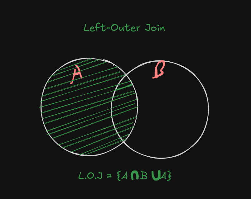
Left-Outer Join returns the matching rows and the rows which are only present in the left table, but not in the right table.
Example 1
Tables:
Employees3
| EmpID | Name | ProjectID |
|---|---|---|
| 201 | Anil | P1 |
| 202 | Sunita | P2 |
| 203 | Rakesh | NULL |
Projects
| ProjectID | ProjectName |
|---|---|
| P1 | Alpha |
| P2 | Beta |
| P3 | Gamma |
🔍 Task:
List all employees along with their project names. If an employee isn't assigned to any project, still show them.
Output:
Select Name, ProjectName FROM Employees3 LEFT OUTER JOIN Projects ON (Employees3.ProjectID = Projects.ProjectID);
+--------+-------------+
| Name   | ProjectName |
+--------+-------------+
| Anil   | Alpha       |
| Sunita | Beta        |
| Rakesh | NULL        |
+--------+-------------+
3 rows in set (0.004 sec)
The ON clause defines the condition used to match rows between two tables when you're performing a JOIN.
Think of it like this:
🔗 "
ONtells SQL how to join the tables — which columns to match rows by."
Example 2:
Tables:
Students2
| StudentID | Name |
|---|---|
| 1 | Alice |
| 2 | Bob |
| 3 | Charlie |
Submissions
| StudentID | Assignment |
|---|---|
| 1 | A1 |
| 2 | A2 |
🔍 Task:
Show all students along with the assignments they submitted. If a student hasn't submitted anything, still include them.
Output:
SELECT Name, Assignment FROM Students LEFT OUTER JOIN Assignments ON (Students.StudentID = Assignments.StudentID);
+---------+------------+
| Name    | Assignment |
+---------+------------+
| Alice   | A1         |
| Bob     | A2         |
| Charlie | NULL       |
+---------+------------+
3 rows in set (0.000 sec)
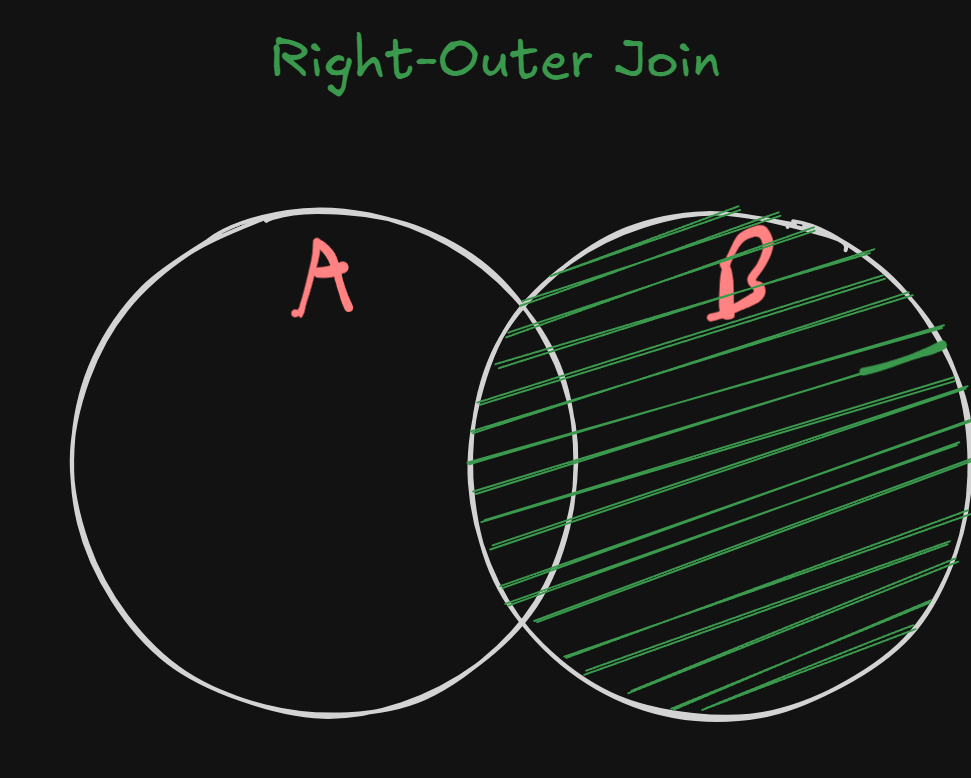
RIGHT OUTER JOIN
Example 1
| EmpID | Name | DeptID |
|---|---|---|
| 101 | Ravi | D1 |
| 102 | Priya | D2 |
departments2
| DeptID | DeptName |
|---|---|
| D1 | HR |
| D2 | IT |
| D3 | Finance |
Perform a right outer join on this table and display the employee names along with their department names.
Output:
SELECT Name, DeptName FROM Employees RIGHT OUTER JOIN Departments ON (Employees.DeptID = Departments.DeptID);
+-------+----------+
| Name  | DeptName |
+-------+----------+
| Ravi  | HR       |
| Priya | IT       |
| NULL  | Finance  |
+-------+----------+
3 rows in set (0.001 sec)
Example 2
students2
| StudentID | Name |
|---|---|
| 1 | Alice |
| 2 | Bob |
assignments2
| StudentID | Assignment |
|---|---|
| 1 | A1 |
| 2 | A2 |
| 3 | A3 |
Perform a right outer join and display the names of the students and their submitted assignments.
Output:
SELECT Name, Assignment FROM Students RIGHT OUTER JOIN Assignments ON (Students.StudentID = Assignments.StudentID);
+-------+------------+
| Name  | Assignment |
+-------+------------+
| Alice | A1         |
| Bob   | A2         |
| NULL  | A3         |
+-------+------------+
3 rows in set (0.000 sec)
🔗 JOIN TYPES COMPARISON
| Join Type | Returns | Matching Required | Missing Side Fills With |
|---|---|---|---|
| INNER JOIN | Only matching rows from both tables | ✅ Required | ❌ Not shown |
| NATURAL JOIN | Like INNER JOIN, but auto-matches columns with same name | ✅ Required | ❌ Not shown |
| EQUI JOIN | INNER JOIN with explicit condition | ✅ Required | ❌ Not shown |
| LEFT OUTER JOIN | All left table rows + matching right rows | ❌ Not always | ✅ Right = NULL if missing |
| RIGHT OUTER JOIN | All right table rows + matching left rows | ❌ Not always | ✅ Left = NULL if missing |
| SELF JOIN | A table joined with itself (can be any join type) | Contextual | Based on condition |
| FULL OUTER JOIN | All rows from both tables (match when possible) | ❌ Not always | ✅ Both sides can be NULL |
🔍 Visual Comparison:
Table A:         Table B:

 A1  A2          B1  B2

    INNER JOIN:
     A ⋈ B       → Matches Only

    NATURAL JOIN:
     A ⋈ B       → Like INNER JOIN, auto-detects join column(s)

    LEFT OUTER JOIN:
     A ⟕ B       → All A, matched B or NULL

    RIGHT OUTER JOIN:
     A ⟖ B       → All B, matched A or NULL

    FULL OUTER JOIN:
     A ⟗ B       → All A + All B, matched or NULL

    SELF JOIN:
     A ⋈ A       → A joins to itself (e.g., employee-manager)
🧠 Mnemonics:
- INNER JOIN = Intersection
- LEFT JOIN = "Give me everything on the left"
- RIGHT JOIN = "Give me everything on the right"
- FULL OUTER JOIN = Union with gaps filled in
- NATURAL JOIN = INNER JOIN but less typing
- SELF JOIN = Compare rows in the same table
Difference between Primary Key, Candidate Key and Super Key.
Among these keys you will hear this phrase quite often:
"Can uniquely identify a row".
So if you are like me who is still confused to as to what this means to this day, here's a clear breakdown which I hope will clear up the meaning of this phrase first.
🔍 What does “uniquely identify a row” mean?
In a table, each row represents one real-world object or entity — like one student, one employee, one order, etc.
To uniquely identify a row means:
You should be able to find one and only one row based on the value(s) in certain column(s).
🧠 Why is this important?
Without unique identification:
- You can’t tell one row from another.
- You can’t update or delete only one specific record reliably.
- Your data can become inconsistent or duplicated.
🧾 Let’s take an example:
📋 STUDENTS Table
| StudentID | Name | |
|---|---|---|
| 101 | Alice | alice@mail.com |
| 102 | Bob | bob@mail.com |
| 103 | Alice | alice123@mail.com |
Let’s now test some columns:
🟥 Case 1: Use only Name to identify a row:
You search for:
"WHERE Name = 'Alice'"
⛔ Result: You get 2 rows. So this does NOT uniquely identify a row.
✅ Case 2: Use StudentID:
You search for:
"WHERE StudentID = 102"
✅ Result: Only 1 row — Bob.
This uniquely identifies the row.
✅ Case 3: Use Email:
"WHERE Email = 'alice@mail.com'"
✅ One row. Also uniquely identifies a row.
So:
StudentID→ Unique → can identify.Email→ Unique → can identify.Name→ Not unique → ❌ can’t identify.
🔑 How does this connect with Keys?
If a column (or combo of columns) can always be used to find one and only one row, it qualifies as a key.
📌 Real-Life Analogy:
Think of a college student list:
- Many students may be named "Rahul Kumar".
- But only one has student ID "20231234".
So even if names repeat, student ID is like a fingerprint — no two students share it.
That's unique identification.
Summary
🟢 A column (or combination) uniquely identifies a row if:
- No two rows ever share the same value(s) in that column(s).
- You can always use it to pinpoint a single, specific row.
Now, I hope that has cleared up what do you mean by "uniquely identifying a row".
So now let's proceed to the keys themselves.
🔑 1. What is a Key in general?
A key is a column (or a set of columns) used to uniquely identify each row in a table.
🔹 2. Super Key – The Superset
A super key is any combination of columns that can uniquely identify rows.
Example:
| StudentID | Name | |
|---|---|---|
| 101 | Alice | alice@mail.com |
| 102 | Bob | bob@mail.com |
| 103 | Charlie | charlie@mail.com |
Possible Super Keys:
{StudentID}{Email}{StudentID, Name}{StudentID, Email}{StudentID, Name, Email}
Note: As long as it uniquely identifies a row, it's a super key. Even if it's got extra unnecessary columns.
🔹 3. Candidate Key – The Minimalist
A candidate key is a minimal super key, meaning:
➤ It still uniquely identifies rows,
➤ But contains no unnecessary columns.
From the table above:
{StudentID}✅ (unique and minimal){Email}✅ (unique and minimal){StudentID, Email}❌ (it's a super key, but not minimal → already uniquely identified by one field)
So here:
- ✅ Candidate Keys =
{StudentID},{Email}
🔹 4. Primary Key – The Chosen One
A primary key is one of the candidate keys that you choose to be the main identifier.
Rules:
- Only one primary key per table.
- Cannot have
NULL. - Must be unique.
So from above, you might pick:
PRIMARY KEY (StudentID)
The others (like Email) remain candidate keys but not the primary.
🔄 Summary Table:
| Term | Is Unique? | Minimal? | Nullable? | Count Per Table |
|---|---|---|---|---|
| Super Key | ✅ | ❌ | ✅ | Many |
| Candidate Key | ✅ | ✅ | ✅ | Many |
| Primary Key | ✅ | ✅ | ❌ | Only One |
🧠 Mnemonic to Remember:
- Super Keys = Super big (can have extra columns)
- Candidate Keys = Candidates for primary key (minimal, unique)
- Primary Key = The picked one from the candidates