Index

1. 1. Relational Algebra
2. 1. Select Operation
3. 2. Project Operation
4. 3. Set Union Operation
5. 4. Set Difference Operation
6. 5. Cartesian Product Operation
7. 6. Rename Operation
8. 2. Relational Calculus
9. 1. Tuple Relational Calculus
10. 2. Domain Relational Calculus
11. 3. SQL basics, SQL3 and it's enhancements
12. 6.2. Armstrong's Axioms (Inference Rules)
13. 7. Normalization
14. 7.1. First Normal Form (1NF)
15. 7.2 Second Normal Form (2NF)
16. What is a partial dependency??
17. How Do We Decide Functional Dependencies (FDs)?
18. 7.3 Third Normal Form (3NF)
19. 7.4 Boyce-Codd Normal Form (BCNF)
20. 11. Join operation and it's types.
21. 2. Natural Join
22. 3. Self Join
23. 4. Equi Join
24. 5. Left-Outer Join
25. 6. Right-Outer Join

1. Relational Algebra

Relational algebra is a procedural query language. It consists of a set of operations that take one or more relations (tables) as input and produce a new relation as output. These operations allow you to express queries in a step-by-step manner.

1.1 Fundamental Operators

• Selection (σ)

  • Purpose: Filters rows based on a specified condition.
  • Notation:
  $${\sigma }_{\text{condition}}(R)$$
  • Example:
    • If $R$ is an Employee table, then

(returns all employees with a salary greater than 50,000.

• Projection (π)

  • Purpose: Extracts specific columns from a relation.
  • Notation:
  $${\pi }_{{\text{column}}_1,{\text{column}}_2,\dots }(R)$$
  • Example:
    • To obtain only the names and departments from Employee, write:

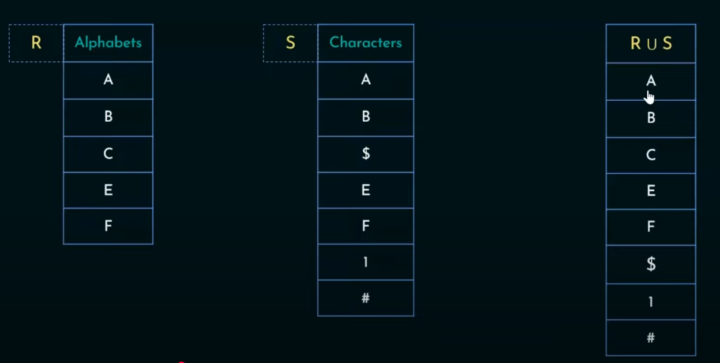
• Union (∪)

  • Purpose: Combines the tuples of two relations that have the same schema, eliminating duplicates.
  • Notation:

- Example:
- Combining two relations R and S that store similar data.

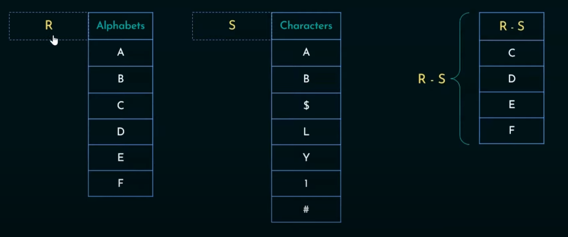
• Set Difference (-)

  • Purpose: Returns tuples that are in one relation but not in another.
  • Notation:

- Example:
- If R is the set of all employees and S is the set of employees in the IT department, then $R-S$ gives you employees not in IT.

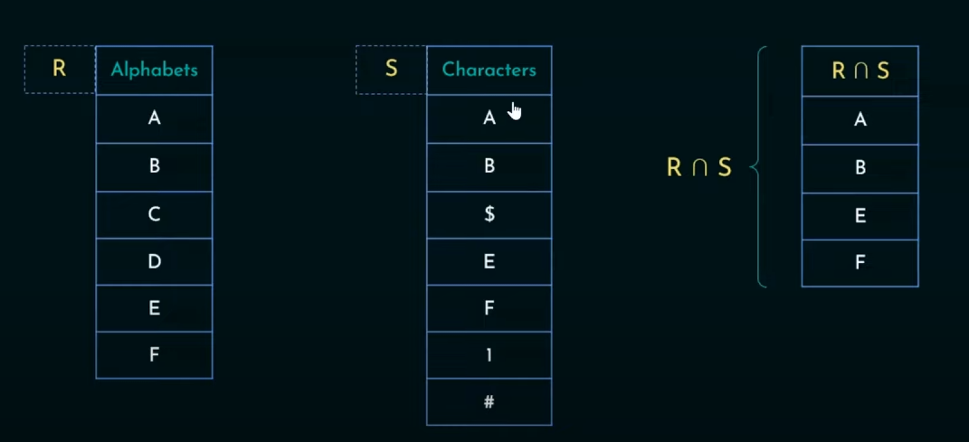
• Intersection (∩)

  • Purpose: Returns only the tuples common to both relations.
  • Note: Intersection can be derived using union and difference:

• Cartesian Product (×)

  • Purpose: Combines every tuple of one relation with every tuple of another relation.
  • Notation:

- Example:
- If R has 3 tuples and S has 4 tuples, then

Worked out examples

1. Select Operation

https://www.youtube.com/watch?v=Givp56x6vbg&list=PLdnwl-gHn1DFIbW82OIyO21lke98MAOKk&index=2

2. Project Operation

https://www.youtube.com/watch?v=QY2X_TlLkqo&list=PLdnwl-gHn1DFIbW82OIyO21lke98MAOKk&index=3

3. Set Union Operation

For Fall 2009 Semester :

For Spring 2010 Semester:

To find the set of them both :

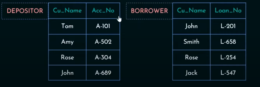
4. Set Difference Operation

https://www.youtube.com/watch?v=dS214kONAZA&list=PLdnwl-gHn1DFIbW82OIyO21lke98MAOKk&index=5

We need to display the customer names which are not in borrower table.

For Fall 2009 Semester :

For Spring 2010 Semester:

For those which were not taught in Spring 2010 :

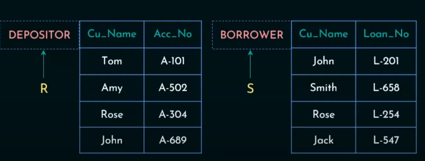
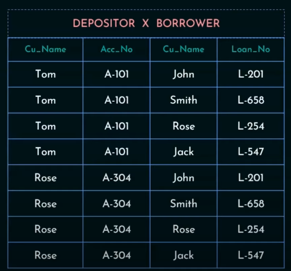
5. Cartesian Product Operation

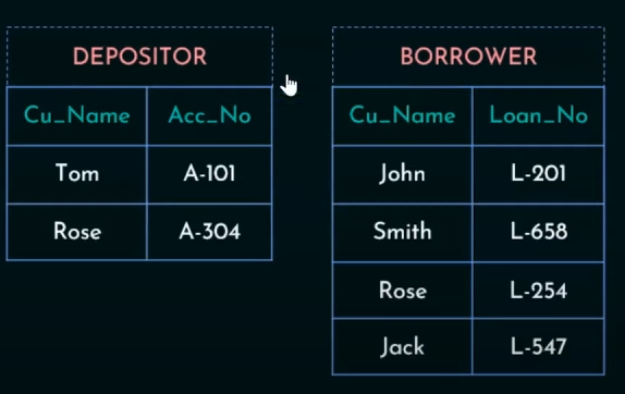
Cartesian Product will map each row of Depositor to each column of Borrower

So output will be:

6. Rename Operation

2. Relational Calculus

Relational calculus is a non-procedural (declarative) query language. Instead of specifying the steps to obtain the result (as in relational algebra), you specify what you want, and the DBMS figures out how to compute it.

2.1 Tuple Relational Calculus (TRC)

https://www.youtube.com/watch?v=zhf3nkoz4ds&list=PLBlnK6fEyqRiyryTrbKHX1Sh9luYI0dhX&index=41

• Concept:
  • TRC uses tuple variables to describe the desired result.
  • A query in TRC has the form: $${t \mid P(t)}$$where $t$ is a tuple variable and $P(t)$ is a predicate (a condition) that $t$ must satisfy.
• Example:
  • To retrieve all employees with a salary over 50,000: $${t \mid t \in \text{Employee} \land t[salary] > 50000}$$
  • Here, $t$ represents each tuple in the Employee relation that meets the condition.

2.2 Domain Relational Calculus (DRC)

https://www.youtube.com/watch?v=BmoZEHPPBoI&list=PLBlnK6fEyqRiyryTrbKHX1Sh9luYI0dhX&index=43

• Concept:
  • DRC uses domain variables that take on values from an attribute’s domain.
  • A query in DRC is expressed as: $${\langle x_1, x_2, \ldots, x_n \rangle \mid P(x_1, x_2, \ldots, x_n)}$$
  • $x_1,x_2,\dots ,x_{n}x$​ represent the values of attributes in the resulting tuple.
• Example:
  • For the Employee table, to get the names and salaries of employees earning more than 50,000: $${\langle n, s \rangle \mid \exists e (e \in \text{Employee} \land e.\text{name} = n \land e.\text{salary} = s \land s > 50000)}$$
  • This states that there exists a tuple $e$ in Employee where the name and salary meet the condition.

2.3 Comparing Relational Algebra and Calculus

• Procedural vs. Declarative:

  • Relational Algebra: You describe how to get the result (step-by-step operations).
  • Relational Calculus: You describe what result you want, leaving the "how" to the DBMS.

• Expressiveness:

  • Both are equivalent in expressive power (each can express the same set of queries), though their styles are different.

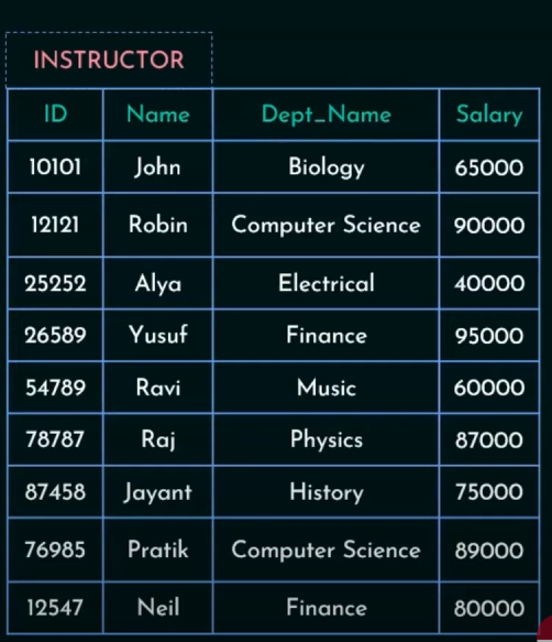
Worked out Examples

1. Tuple Relational Calculus

So we are asked to retrieve the ID only.

In this case, we will use an existential quantifier.

It will be of this format :

which reads as "there exists a tuple t in a relation r", then the predicate (Q(t)) should be true.

$t$ is the list of all tuples retrieved from the table.

So our solution will be :

which reads as "there exists a tuple s in the relation, that being ID of t equals ID of s and salary is greater than eighty thousand".

Note that the data asked in the question was not in the table so we will proceed with some assumptions.

And for department we will use another tuple variable, that belongs to the department relation

So it will be

$\{t|\mathrm{\exists }s\in instructor(t[Name]=s[Name]\wedge \mathrm{\exists }u\in department(u[\text{dept-name}]=s[\text{dept-name}]\wedge u[building]="Watson"))\}$

For Fall 2009 Semester :

For Spring 2010 Semester :

Together in the "OR" format :

$\{t|\mathrm{\exists }s\in section(t[\text{course-id}]=s[\text{course-id}])\wedge s[Semester]="Fall"\wedge s[Year]=2009\}\vee$ $\{t|\mathrm{\exists }u\in section(t[\text{course-id}]=u[\text{course-id}])\wedge u[Semester]="Fall"\wedge u[Year]=2009\}$

Same just now we need to find both of them together, so we use conjunction (AND) instead of disjunction (OR)

$\{t|\mathrm{\exists }s\in section(t[\text{course-id}]=s[\text{course-id}])\wedge s[Semester]="Fall"\wedge s[Year]=2009\}\wedge$ $\{t|\mathrm{\exists }u\in section(t[\text{course-id}]=u[\text{course-id}])\wedge u[Semester]="Fall"\wedge u[Year]=2009\}$

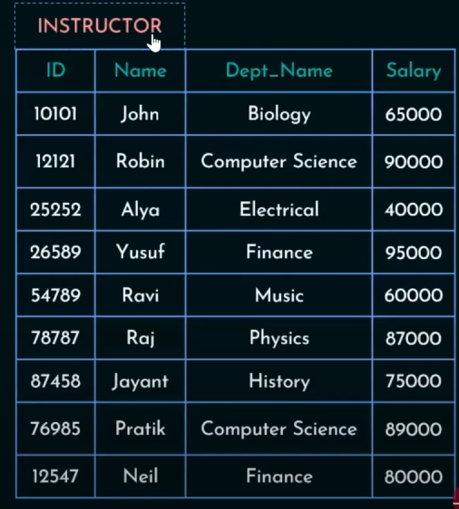
2. Domain Relational Calculus

In domain relational calculus instead of dealing with entire row tuples, we deal with the column attributes.

So in this case, the attributes are ID, Name, Dept_Name and Salary, which can be represented in short as i, n, d and s

So the solution will be:

Since we only have to find the ID from this table, we will use an existential quantifier.

In this form:

which says that "there exists a variable x which satisfies the given predicate $P_1(x)$"

So it would be this way:

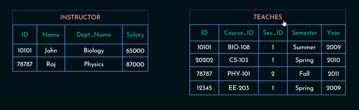
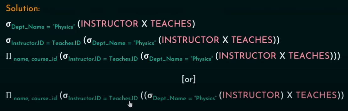
So we need to work with two tables, Instructor and Teaches.

For first table we only need the Name field.

$\{<n,c>|\mathrm{\exists }i,a(<i,c,a,s,y>\in Teaches\wedge \mathrm{\exists }d(<i,n,d,s>\in Instructor\wedge \text{Dept-Name}="Physics"))\}$
Here $a$ is selected for sec_id and $s$ is not used here to avoid ambiguity for using two same variables one after another.

$\{<c>|\mathrm{\exists }s(<c,a,s,y,b,r,t>\in Section\wedge s="Fall"\wedge y=2009)\vee \mathrm{\exists }u(<c,a,s,y,b,r,t>\in Section\wedge s="Spring"\wedge y=2010)\}$

3. SQL basics, SQL3 and it's enhancements

Part 1: SQL Basics

SQL (Structured Query Language) is the standard language for interacting with relational databases.

1.1 Overview of SQL

• Purpose:
  SQL is used for creating, managing, and querying data in relational databases.
• Key Components:
  • DDL (Data Definition Language): Commands that define or alter the structure of the database (e.g., CREATE, ALTER, DROP).
  • DML (Data Manipulation Language): Commands that operate on the data itself (e.g., INSERT, UPDATE, DELETE, SELECT).
  • DCL (Data Control Language) and TCL (Transaction Control Language): Commands that control access and manage transactions.

1.2 SQL3 and Its Enhancements

• SQL3:
  Often referred to as the third generation of SQL standards, SQL3 extended traditional SQL with object-oriented features, such as:

  • User-defined types: Allowing custom data types.
  • Inheritance: Enabling a form of class hierarchies in databases.
  • Enhanced integrity constraints: More robust ways to ensure data consistency.

• Real-World Note:
  Although many databases support a core SQL standard, different DBMSs have their own extensions. It’s useful to be familiar with these differences.

1.3 SQL DDL: Creating and Modifying Database Structures

CREATE Statement

• Purpose: Define a new database object, such as a table.

• Example: Creating a table for a student database:

CREATE TABLE Students (
    student_id INT PRIMARY KEY,
    name VARCHAR(50) NOT NULL,
    major VARCHAR(50),
    enrollment_date DATE,
    CHECK (enrollment_date <= CURRENT_DATE)
);

ALTER Statement

• Purpose: Modify an existing database object (e.g., add a column).

• Example: Adding an email column to the Students table:

ALTER TABLE Students
    ADD COLUMN email VARCHAR(100);

DROP Statement

• Purpose: Remove an object from the database.

• Example: Dropping the Students table:

DROP TABLE Students;

TRUNCATE Statement

• Purpose: Quickly remove all rows from a table, often faster than deleting each row individually.

• Example:

TRUNCATE TABLE Students;

1.4 SQL DML: Managing and Querying Data

INSERT Statement

• Purpose: Add new records to a table.

• Example:

INSERT INTO Students (student_id, name, major, enrollment_date, email)
VALUES (101, 'Alice Johnson', 'Computer Science', '2023-08-20', 'alice@example.com');

UPDATE Statement

• Purpose: Modify existing records.

• Example:

UPDATE Students
SET major = 'Software Engineering'
WHERE student_id = 101;

DELETE Statement

• Purpose: Remove records from a table.

• Example:

DELETE FROM Students
WHERE student_id = 101;

SELECT Statement

• Purpose: Retrieve data from one or more tables.

• Basic Example:

SELECT student_id, name, major
FROM Students
WHERE major = 'Computer Science';

• Advanced Techniques:

  • JOINs: Combining data from related tables.
  • Aggregations: Using functions like COUNT(), SUM(), AVG().
  • Subqueries: Nesting queries within other queries.

5. Types of DBMS software

DBMSs come in various types, each with unique strengths. They generally fall into two broad categories: Open Source and Commercial. Additionally, within these categories, there are differences based on the underlying technology and features.

2.1 Open Source DBMS

• Examples:
  • MySQL: Widely used for web applications; known for its speed and ease of use.
  • PostgreSQL: Known for its standards compliance and advanced features (e.g., support for custom data types, robust ACID compliance).
• Advantages:
  • No licensing fees.
  • Strong community support.
  • Rapid development cycles and frequent updates.
• Use Cases:
  Web development, small to medium-scale applications, and academic projects.

2.2 Commercial DBMS

• Examples:
  • Oracle Database: Known for its advanced features, scalability, and robust support for enterprise applications.
  • Microsoft SQL Server: Offers strong integration with other Microsoft products, comprehensive tools, and ease of management.
  • IBM DB2: Popular in large enterprises, known for its reliability and performance.
• Advantages:
  • Comprehensive support and services.
  • Advanced performance tuning, security features, and scalability.
  • Often comes with enterprise-grade tools for backup, recovery, and data analytics.
• Use Cases:
  Large-scale enterprise applications, mission-critical systems, and environments requiring stringent security and high availability.

2.3 Key Differences and Considerations

• Licensing and Cost:
  Open source solutions are free to use and modify, whereas commercial DBMSs require licensing fees.
• Support and Community:
  Commercial DBMSs offer professional support, while open source systems rely on community forums and contributions.
• Feature Set:
  Commercial systems often include additional features such as advanced replication, clustering, and integrated analytics.
• Performance and Scalability:
  While many open source DBMSs are highly performant, commercial systems are typically optimized for extremely high workloads and large-scale deployments.

6. Relational Database Design

6.1. Domain and Data Dependency

1.1 Domain

• Definition:
  A domain is the set of all possible values an attribute can have. For example, for an attribute age, the domain might be all positive integers within a reasonable range (e.g., 0–150).

• Purpose:
  It ensures data integrity by restricting values to what’s meaningful (e.g., a gender field might be limited to {‘M’, ‘F’, ‘Other’}).

1.2 Data Dependency

• Definition:
  Data dependency describes how one attribute’s value depends on another. This is the basis for functional dependency.

• Functional Dependency Example:
  In a student database, if the student’s ID uniquely determines the student’s name and birth date, we express it as:

6.2. Armstrong's Axioms (Inference Rules)

Armstrong’s Axioms provide a sound and complete set of rules to infer all functional dependencies from a given set. There are three primary axioms:

2.1 Reflexivity (Trivial Dependency)

• Statement:
  If $Y$ is a subset of $X$ (written $Y\subseteq X$), then $X\to Y$.
• Intuition:
  An attribute set always functionally determines its own subset. This is obvious because if you know all the attributes in $X$, you certainly know any subset of those attributes.
• Example:
  Consider $X=\{A,B\}$ . Since $\{A\}\subseteq \{A,B\}$, by reflexivity, we have: $\{A,B\}\to \{A\}$
• Significance:
  Reflexivity is the most basic rule; it confirms that no extra information is needed to determine part of what you already have.

2.2 Augmentation

• Statement:
  If $X\to Y$ holds, then for any set of attributes $Z$, the dependency $XZ\to YZ$ also holds.
• Intuition:
  If you know $X$ determines $Y$, then if you add more attributes $Z$ to both sides, knowing $X$ and $Z$ still guarantees you know $Y$ and $Z$. Adding extra information does not remove the dependency.
• Example:
  Suppose we have the dependency: $\{A\}\to \{B\}$ If we augment both sides with another attribute $C$, we get: $\{A,C\}\to \{B,C\}$
• Application Tip:
  This rule is often used when combining dependencies or when the context of a query or design requires additional attributes to be included.

2.3 Transitivity

• Statement:
  If $X\to Y$ and $Y\to Z$ hold, then $X\to Z$ also holds.

• Intuition:
  Think of it as a chain reaction: if knowing $X$ gives you $Y$, and knowing $Y$ $gives you $Z$, then knowing $X$ should give you $Z$ indirectly.

• Example:
  Assume:

  • $\{A\}\to \{B\}$
  • $\{B\}\to \{C\}$
    Then by transitivity,

  $\{A\}\to \{C\}$

• Real-World Analogy:
  Consider a university database where $A$ is a student's ID, $B$ is the student's major, and $C$ is the department head for that major. If a student's ID determines their major, and the major determines the department head, then the student's ID indirectly determines the department head.

6.3. Derived Inference Rules

Using Armstrong's basic axioms, we can derive additional useful rules. These are not independent of the three axioms but are convenient shortcuts.

3.1 Union Rule (Additivity)

• Statement:
  If $X\to Y$ and $X\to Z$, then $X\to Y\cup Z$.

• Example:
  Suppose:

  • $\{A\}\to \{B\}$
  • $\{A\}\to \{C\}$

  Then:

  $\{A\}\to \{B,C\}$

• Justification:
  Both dependencies ensure that $A$ determines $B$ and $C$ separately, so together $A$ determines both $B$ and $C$.

3.2 Decomposition Rule (Projectivity)

• Statement: If $X\to YZ$ holds, then $X\to Y$ and $X\to Z$ holds separately.

• Example:

  Given:

  $$\{A\}\to \{B,C\}$$

  It follows that:

  $\{A\}\to \{B\}$
  $\{A\}\to \{C\}$

• Usage:

  This rule is useful when you need to analyze or simplify dependencies by breaking them into smaller parts.

3.3 Pseudotransitivity

• Statement:

  If $X\to Y$ and $WY\to Z$ hold, then $XW\to Z$ holds.

• Example:

  Suppose :

  $$\{A\}\to \{B\}$$

  and

  $$\{C,B\}\to \{D\}$$

  Then, by pseduotransitivity:

  $$\{A,C\}\to \{D\}$$

• Intuition:

  It’s an extension of transitivity that allows for extra attributes $W$ to be added to the determinant if those attributes already accompany the dependent in the second dependency.

6.4. Practical Applications in Database Design

Understanding and applying Armstrong’s axioms is crucial during the normalization process in database design:

• Normalization:

  • Identifying Candidate Keys: By analyzing functional dependencies using these axioms, you can determine the minimal sets of attributes (candidate keys) that uniquely identify a row.

  • Decomposing Relations: You ensure that tables are split in a way that minimizes redundancy and prevents anomalies (like update or insertion anomalies) by maintaining proper functional dependencies.

    Normalization is done in the following sections.

• Query Optimization:
  Knowing the functional dependencies allows the database management system (DBMS) to optimize queries by understanding which attributes determine others.

Worked-out Example

Imagine a relation $R(A,B,C,D)$ with the following functional dependencies:

1. $A\to B$
2. $B\to C$
3. $A,D\to C$

Step-by-Step Analysis:

1. Reflexivity check: Since $A$ depends on $B$ this means that $B\subseteq A$

2. Augmentation:

   • From $A\to B$ , if we augment both sides with an arbitrary attribute, let's say $Z$, then :

     $$\{A,Z\}\to \{B,Z\}$$

3. Transitivity:

   Since $A\to B$ and $B\to C$ then using transitivity we get: $A\to C$

4. Pseudotransitivity Check:

   Since $A\to B$ , $B\to C$, thus $A\to C$.

   So A and B are interchangeable.

   So $A,D\to C$, can become $B,D\to C$

   Now from pseduotransitivity, we reconfirm that :

   Since $A\to C$ and $B,D\to C$, we can treat D here as an extra attribute (W).

   So by pseduotransitivity we get $A,D\to C$.

• This is consistent with the original dependency provided.

These steps help confirm the correctness of the given dependencies and also assist in deriving additional dependencies if needed.

6.5. Summary

• Armstrong’s Axioms provide a rigorous, logical foundation for inferring functional dependencies.
• Reflexivity confirms that an attribute set determines its own subsets.
• Augmentation shows that extra information added to both sides of a dependency does not change the dependency.
• Transitivity enables chaining of dependencies to derive indirect relationships.
• Derived rules (union, decomposition, pseduotransitivity) offer practical shortcuts for database design and normalization.

7. Normalization

Normalization is a systematic approach to organizing data in a database to minimize redundancy and avoid undesirable anomalies during data operations (insertion, update, deletion). It involves decomposing a table into smaller, well-structured tables while preserving data integrity and ensuring that relationships among the data remain clear. Let’s explore normalization in detail, focusing on the most common normal forms:

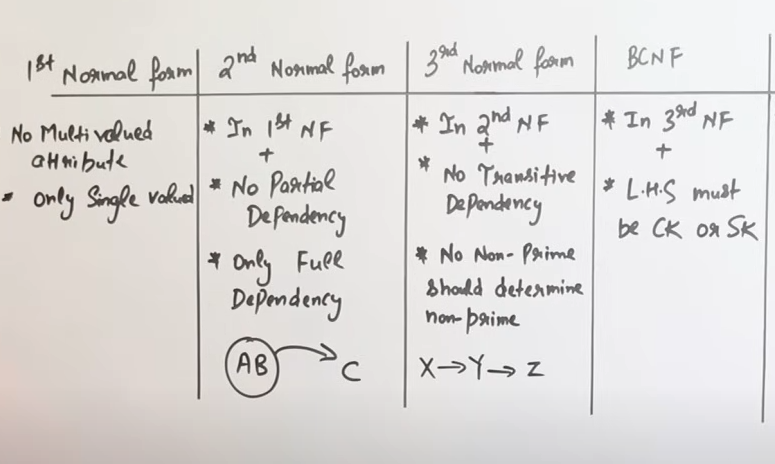
7.1. First Normal Form (1NF)

Definition

A relation (table) is in 1NF if:

• Atomicity: Every cell in the table contains a single (atomic) value. No cell should contain sets, lists, or multiple values.
• No Repeating Groups: The table does not contain repeating groups or arrays.

Why 1NF?

• Simplicity: Ensures that each piece of data is stored in a single cell, which simplifies querying and updating the data.
• Foundation for Further Normalization: Being in 1NF is the baseline requirement before considering more advanced normal forms.

Example

Imagine a table of students with a column that stores multiple phone numbers:

To convert this into 1NF, you’d separate the phone numbers so that each cell holds only one value:

7.2 Second Normal Form (2NF)

https://www.youtube.com/watch?v=tkbAA--wKOc&list=PLxCzCOWd7aiFAN6I8CuViBuCdJgiOkT2Y&index=25

Definition

A table is in 2NF if:

• It is already in 1NF.
• Every non-prime attribute (i.e., an attribute that is not part of any candidate key) is fully functionally dependent on the entire primary key. This means that if you have a composite primary key (a key made up of more than one attribute), no non-key attribute should depend on only part of that key (partial dependency).

Recap of keys :

Super Key

• Definition: A super key is any set of one or more attributes that can uniquely identify a row (tuple) in a table.
• Key Point: It might include extra attributes that are not necessary for unique identification.
• Example: In a table with attributes {StudentID, Email, Phone}, the set {StudentID, Email} is a super key even if just {StudentID} is enough.

Candidate Key

• Definition: A candidate key is a minimal super key. That means it is a set of attributes that uniquely identifies each row, and no proper subset of this key can uniquely identify the row.
• Key Point: A table can have multiple candidate keys.
• Example: If both {StudentID} and {Email} uniquely identify students, each is a candidate key. Neither contains extra attributes.

Primary Key

• Definition: A primary key is a candidate key that has been chosen by the database designer to uniquely identify records in the table.
• Key Point: There can be only one primary key per table, and it must not allow null values.
• Example: If both {StudentID} and {Email} are candidate keys, the designer might choose {StudentID} as the primary key.

Composite Primary Key

• Definition: A composite primary key is simply a primary key that consists of more than one attribute.
• Key Point: It is used when no single attribute can uniquely identify the records on its own.
• Example: In an order detail table, a combination of {OrderID, ProductID} might be used as the composite primary key because neither alone is sufficient to uniquely identify each record.

Summary Comparison

• Super Key vs. Candidate Key:
  • Super Key: May contain redundant attributes.
  • Candidate Key: Is minimal (no unnecessary attributes).
• Candidate Key vs. Primary Key:
  • Candidate Key: There can be multiple; all are minimal super keys.
  • Primary Key: One candidate key is chosen as the main unique identifier.
• Primary Key vs. Composite Primary Key:
  • Primary Key: Can be a single attribute or a combination.
  • Composite Primary Key: Specifically refers to a primary key that uses more than one attribute.

Why 2NF?

• Eliminates Partial Dependencies: This prevents redundancy that can occur when non-key attributes depend on only a portion of a composite key.

Example

Consider a table storing student enrollments:

Here, the composite key is $\{studentid,courseid\}$. Notice that:

• student_name depends only on student_id.
• course_name depends only on course_id.

To remove these partial dependencies, decompose the table into three:

Student Table:

Course Enrollment Table:

Course Table:

Understanding the steps in detail.

Step 1. List all attributes and the functional dependencies.

So in this table we have the attributes as:

• student_id
• course_id
• student_name
• course_name

Now for the functional dependencies :

How Do We Decide Functional Dependencies (FDs)?

https://www.youtube.com/watch?v=qn5neFBpU40&list=PLxCzCOWd7aiFAN6I8CuViBuCdJgiOkT2Y&index=24

Not solely based on 1:1 relationships.

• Functional Dependencies come from the semantics or rules of the real-world domain.
• For example, if every student has one unique name, then:
  • $\text{student\_id}\to \text{student\_name}$
    means that for any given student_id, you always get the same student_name.
• In contrast, a student may enroll in many courses (a one-to-many relationship), so you wouldn’t have $\text{student\_id}\to \text{course\_id}$ can be associated with multiple $course\mathrm{\_}id$ s.

Key point:
FDs are determined by how the data logically relates—not just by whether relationships are 1:1. Sometimes, even in a one-to-many or many-to-many scenario, you still have FDs for the parts that are 1:1 (e.g., student_id → student_name or course_id → course_name).

Functional dependencies also have the properties of Armstrong's axioms

This is done by first identifying the domain rules

So in our original table we have :

So we identify the functional dependencies first :

$student\mathrm{\_}id\to course\mathrm{\_}id$ (not valid in this case since there is a student with a same id enrolling in two different courses)
$course\mathrm{\_}id\to student\mathrm{\_}name$ (not valid since there is no point in linking a course id to a student's name)
$student\mathrm{\_}name\to course\mathrm{\_}name$ (not valid since it implies that a student can only take one course where already student id points to multiple course ids)
$student\mathrm{\_}id\to student\mathrm{\_}name$ (from transitivity)
$student\mathrm{\_}id\to course\mathrm{\_}name$ (from transitivity) (not valid in this case since a single student can take multiple courses)
$course\mathrm{\_}id\to course\mathrm{\_}name$ (from transitivity)

student_id -> student_name
course_id -> course_name

Step 2: Find candidate key by performing closure on functional dependencies

https://www.youtube.com/watch?v=bSdvM_0hzgc&list=PLxCzCOWd7aiFAN6I8CuViBuCdJgiOkT2Y&index=23

So we have a relation as $R(A,B,C,D)$

Let $A$ = $student\mathrm{\_}id$ ; $B=course\mathrm{\_}id$ ; $C=student\mathrm{\_}name$ ; $D=course\mathrm{\_}name$

So the functional dependencies will be :

$A\to C$
$B\to D$

So we start by finding the closure of A

For B :

So if we group A and B and take closure of AB

Now while finding Candidate keys it is a good practice to check other possible combinations of candidate keys.

As we see here:

$C^{+}=\{C\}$
$D^{+}=\{D\}$

$A{C}^{+}=\{C,A\}$
$A{D}^{+}=\{A,D\}$
$B{D}^{+}=\{B,D\}$
$B{C}^{+}=\{B,D,C\}$

So we see that the closure of AB results in all the attributes of relation R.

So the candidate key will be $AB$ or $\{student\mathrm{\_}id,course\mathrm{\_}id\}$

Step 3: Identify non-prime attributes and partial dependencies

Non-prime attributes are the attributes which are not involved in the formation of the candidate key.

In this instance the non-prime attributes are $student\mathrm{\_}name$, $course\mathrm{\_}name$

Now for the partial dependencies :

What is a partial dependency??

A partial dependency occurs when a non-prime attribute is dependent on only a part of a candidate key, not the whole.

We see from the table that :

$student\mathrm{\_}name$ relates to $student\mathrm{\_}id$ only which is just a part of the candidate key.

$course\mathrm{\_}name$ relates to $course\mathrm{\_}id$ only which is just a part of the candidate key.

So there are two partial dependencies happening here.

Or a short way of identify partial dependencies are if :

LHS of F.D is a proper subset of Candidate Key (i.e part of candidate key, not the whole candidate key itself)

or

RHS of F.D is a non-prime attribute.

Sometimes we need to check for both of these conditions to find out a partial dependency.

Step 4: Separate the table out based on the partial dependencies

To ensure that there are no partial dependencies, we split the original table into three separate tables

Course enrollment table, containing both parts of the candidate key.

Student table where $student\mathrm{\_}name$ fully depends on the candidate key $student\mathrm{\_}id$ .

Course table where $course\mathrm{\_}name$ fully depends on candidate key $course\mathrm{\_}id$ ,

Now this in 2NF form where the tables are already in 1NF form and all non-prime attributes are fully dependent on the candidate key.

7.3 Third Normal Form (3NF)

https://www.youtube.com/watch?v=IeSai2JVm78&list=PLxCzCOWd7aiFAN6I8CuViBuCdJgiOkT2Y&index=26

Definition

A table is in 3NF if:

• It is in 2NF.
• There are no transitive dependencies for non-prime attributes. A transitive dependency exists when a non-key attribute depends on another non-key attribute rather than directly on the primary key.

Why 3NF?

• Reduces Redundancy Further: Eliminating transitive dependencies minimizes redundancy and ensures that every non-key attribute is directly dependent on the primary key.

Example

Consider a table that stores student information along with their advisor and the advisor's office location:

Here, while student_id uniquely determines student_name, it also determines advisor, and advisor determines advisor_office. The dependency $$student_id \rightarrow advisor \rightarrow advisor_office$$

To achieve 3NF, decompose the table:

Student Table:

Advisor Table:

7.4 Boyce-Codd Normal Form (BCNF)

https://www.youtube.com/watch?v=mf_PbWPo7VM&list=PLxCzCOWd7aiFAN6I8CuViBuCdJgiOkT2Y&index=27

Definition

A table is in BCNF if:

• For every non-trivial functional dependency $X\to Y$, $X$ is a candidate key/superkey. (A superkey is an attribute or set of attributes that uniquely identifies a tuple.)

What are trivial and non-trivial functional dependencies??

Trivial Dependency

A functional dependency $X\to Y$is trivial if the set $Y$ is a subset of $X$. In other words, the dependency does not provide any new information because the dependent attributes are already part of the determinant.

• Example:

  Consider a relation $R(A,B,C)$

  • The dependency $\{A,B\}\to A$ is trivial since $A$ is already in $\{A,B\}$
  • Similarly, $\{A,B\}\to \{A,B\}$ is trivial.

Non-trivial Dependency

A functional dependency $X\to Y$ is non-trivial if Y is not a subset of X. This means that $X$ determines some attribute(s) that are already not included in $X$, thereby adding new information.

• Example:

  Again, consider the relation $R(A,B,C)$.

  • The dependency $A\to B$ is non-trivial because $B$ is not a part of $A$.
  • Similarly, $\{A\}\to \{B,C\}$ is non-trivial if neither $B$ nor $C$ is in $A$.

Why BCNF?

• Stricter Requirement: BCNF is a stricter version of 3NF and further reduces redundancy in cases where 3NF still allows certain anomalies.
• Ensures Every Determinant is a Candidate Key: This helps maintain consistency and prevents potential anomalies in complex schemas.

Example

Consider a table with the following dependencies:

Suppose:

• Each course is taught by a specific instructor.
• However, each room can host multiple courses, but an instructor is tied to a room for a given course.
• If we have a dependency like $\{course,room\}\to instructor$, but neither course nor room alone is a superkey, then the table may violate BCNF.

To achieve BCNF, you might need to decompose the table further so that every determinant is a candidate key. The exact decomposition depends on the specific functional dependencies involved.

Summary of all normal forms

https://www.youtube.com/watch?v=EGEwkad_llA&list=PLxCzCOWd7aiFAN6I8CuViBuCdJgiOkT2Y&index=30 (Ignore 4NF and 5NF as those are out of syllabus)

https://www.youtube.com/watch?v=wTJjpH2RUcQ&list=PLxCzCOWd7aiFAN6I8CuViBuCdJgiOkT2Y&index=33

7.5. Advantages and Trade-Offs of Normalization

Advantages:

• Eliminates Redundancy: Reduces data duplication, saving storage and reducing the chance for inconsistencies.
• Prevents Anomalies: Helps avoid update, insert, and delete anomalies that can lead to data corruption.
• Improves Data Integrity: Enforces clear rules about how data relates, ensuring consistent and valid data.

Trade-Offs:

• Complexity in Querying: Highly normalized databases often require multiple joins to retrieve data, which can affect performance and query complexity.
• Overhead of Decomposition: Managing many smaller tables might add overhead in terms of database design and maintenance.
• Performance Considerations: In some cases, a denormalized design is deliberately used in data warehousing or reporting systems for performance reasons, even though it introduces some redundancy.

8. Query Processing

1. Overview of Query Processing

When a user submits an SQL query, the DBMS performs several key steps before returning the results. The process generally involves:

• Parsing:
  The query is checked for syntax errors and is converted into an internal representation.

• Translation into Relational Algebra:
  The parsed query is translated into an equivalent relational algebra expression that captures the logical operations (selection, projection, joins, etc.).

• Query Rewriting:
  Using rules (often based on algebraic equivalences and heuristics), the query is rewritten into an equivalent form that might be more efficient to execute.

• Optimization:
  The query optimizer evaluates multiple possible execution plans. It estimates the cost (e.g., I/O, CPU usage) of each plan based on available statistics. The optimizer then chooses the most efficient plan.

• Execution:
  The chosen physical plan is executed by the DBMS engine, which retrieves the data and returns the results to the user.

9. Relational Algebra and Query Equivalence

Relational algebra provides a formal foundation for query processing. Through a set of operations (like selection, projection, and joins), we can express SQL queries in a mathematical form.

• Example of an Algebra Expression:

  Consider a query joining two relations, Employee and Department, on a common attribute (department_id):

  ${\pi }_{\text{name, dept\_name}}({\sigma }_{Employee.dept\mathrm{\_}id=Department.dept\mathrm{\_}id}(Employee\times Department))$

• Query Equivalence:

  Many different relational algebra expressions can yield the same result. For instance, a join can be expressed as a combination of Cartesian product and selection. The optimizer rewrites the query to choose an expression that minimizes cost.

Equivalence of Functional dependencies

https://www.youtube.com/watch?v=eIXC6NfKno4&list=PLxCzCOWd7aiFAN6I8CuViBuCdJgiOkT2Y&index=36 (Equivalence of Functional dependencies)

So basically we check the equivalence of two functional dependencies by checking if let's say we have two relations $X$ and $Y$, so we check whether these two are equivalent to each other if

$X$ covers $Y$ i.e $X\subseteq Y$ AND $Y$ covers $X$ i.e $Y\subseteq X$ or

$X^{+}$ = $Y^{+}$

Example 1 :

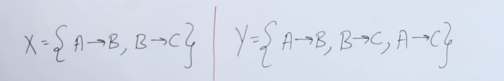
So we have two relations :

$X=\{A\to B,B\to C\}$
$Y=\{A\to B,B\to C,A\to C\}$

So first we need to check if $X$ covers $Y$.

So we start with the closure of the attributes of $X$.

$A^{+}=\{A,B,C\}$
$B^{+}=\{B,C\}$

In the attributes of $Y$ we see that, from $X$, $A$ derives $B$ and $C$. $B$ derives $C$ as well.

So $X$ covers $Y$ or $X\subseteq Y$

Now to check if $Y$ covers $X$.

$A^{+}=\{A,B,C\}$
$B^{+}=\{B,C\}$

So we see that in the attributes of $X$, from $Y$, $A$ derives both $B$ and $C$. And $B$ derives $C$ as well.

So $Y$ covers $X$ or $Y\subseteq X$.

So, since both $X$ and $Y$ cover each other, we can say that $X=Y$ or both the functional dependencies are equivalent.

10. Dependency Preserving Decomposition (Lossless decomposition)

https://www.youtube.com/watch?v=0oeap0QDslY&list=PLxCzCOWd7aiFAN6I8CuViBuCdJgiOkT2Y&index=37

So when we normalize relations and break them down (decompose) into further smaller tables and relations, we must ensure that all the original attributes are present in the decomposed tables such that taking a union of all the decomposed tables will result in all the original attributes from the table.

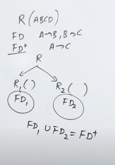
So if we have a relation $R(ABCD)$ and it's decomposed into two children tables $R_1$ and $R_2$ then the decomposition should be in such a way that $R_1\cup R_2$ results in the attributes of $R$.

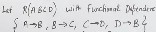
So let's say we have this relation $R$ with the given F.Ds

• $A\to B$
• $B\to C$
• $C\to D$
• $D\to B$

If we were to splice this into three sub tables $R_1$, $R_2$ and $R_3$

The rules would be as follows :

• The selected F.D should not have trivial attributes (i.e $LHS\cap RHS\ne LHS$)
• The selected F.D should actually be valid (i.e it should be directly present in $R$ or be derivable via transitive property).

So Let's say in $R_1$

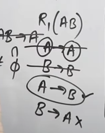
We initially write a bunch of F.Ds

• $A\to A$
• $B\to B$
• $A\to B$
• $B\to B$

Now immediately we see that in $A\to B$ and $B\to B$, these are trivial attributes.

So these won't be considered.

For $A\to B$ it's present in $R$ so it's considered in $R_1$.
$B\to A$ is neither directly present not derivable via transitive property so it's not considered.

Similarly for tables $R_2$ and $R_3$

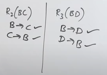
For $R_2$

$B\to C$ works as it's directly given in $R$.

$$\begin{gathered} C\to D;D\to B; \\ C\to B \end{gathered}$$ works

For $R_3$

$B\to C;C\to D;B\to D$ works.

$D\to B$ works as it's directly given in $R$

And now if we were to take a union, i.e $R_1\cup R_2\cup R_3$

it would result in : $\{A\to B,B\to C,C\to B,B\to D,D\to B\}$

Now checking our original set $R$

We see if this union covers $R$ (is equivalent to R)

So :

$A\to B$ present in $R$, works
$B\to C$ present in $R$, works
$C\to B$, not directly present in R, but derivable by transitive property, so it works.
$B\to D$, not directly present in R, but derivable by transitive property, so it works.
$D\to B$ present in R, works.

So the decomposition of $R$ into $R_1$, $R_2$ and $R_3$ was a successful lossless decomposition.

https://www.youtube.com/watch?v=jxENwUU9j7w&list=PLxCzCOWd7aiFAN6I8CuViBuCdJgiOkT2Y&index=38 (Example 2)

11. Join operation and it's types.

https://www.youtube.com/watch?v=zYH-e6tUYbw&list=PLxCzCOWd7aiFAN6I8CuViBuCdJgiOkT2Y&index=39

Joins are fundamental operations in relational databases that allow you to combine rows from two or more tables based on a related column between them. There are several join techniques—each with its own algorithm, performance characteristics, and use cases. Let’s break down the concept and study the major types of joins in detail.

1. What Is a Join?

A join operation merges tuples (rows) from two tables by matching values of one or more common attributes (columns). For example, if you have an Employee table and a Department table, you might join them on a shared attribute like department_id to retrieve each employee along with their department details.

Joins can be categorized in two ways:

• Logical Join Types:
  These define what kind of results you want, such as inner joins, left outer joins, right outer joins, and full outer joins.

• Physical Join Algorithms:
  These define how the join is performed under the hood. We'll focus on these as they relate directly to query processing and optimization.

For our syllabus we only have the following join types

• Natural Join
• Self Join
• Equi Join
• Left Outer Join
• Right Outer Join

2. Natural Join

https://www.youtube.com/watch?v=jRxEjmjIIFs&list=PLxCzCOWd7aiFAN6I8CuViBuCdJgiOkT2Y&index=40

A natural join is a standard join operation involving two tables, where we join the two tables via their cross product and fetch some data from the cross product based on some condition.

The cross product is basically the Cartesian Product operation.

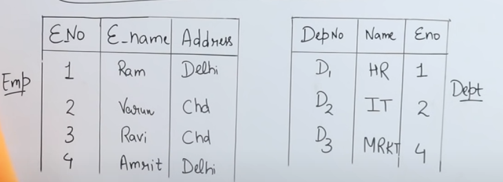
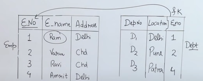
Let's say we have these two tables here.

And we have been tasked to find the employee names who are working in a department.

As the image above says:

And the second condition for a join to be possible is that both tables must have a common attribute.

So we see that $E_{No}$ is a common attribute in both the tables.

So we will start with the cross product :

SELECT E_Name from emp, dept

This is the first part of the Join. Now we need the condition.

We do this as follows :

SELECT E_Name from emp, dept WHERE emp.E_Name = dept.E_name

So this way we will fetch the names of all the employees from the employee table which are assigned to a department in the department table.

So the output table will be :

Note that :

Employee number 3 Ravi was not assigned to any departments so he wasn't fetched in the Join operation.

Now the original way to write this query would be:

SELECT E_Name from emp Natural Join dept

Here we skip writing the condition since we are using the Natural Join operator straightaway.

3. Self Join

https://www.youtube.com/watch?v=6DQpvfdj6EE&list=PLxCzCOWd7aiFAN6I8CuViBuCdJgiOkT2Y&index=41

Now let's say that we have this table right here :

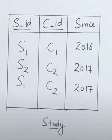
And we are given this task :

Now we see that there's a problem, that we have only 1 table. And a typical join operation works on a cross product that involves two tables. So how do we solve this dilemma?

Simple, we use an "alias". (pronounced "a-lee-us"). We create two aliases of the same table, essentially resulting in two separate copies of the same table.

So we do that using :

SELECT _ FROM Study as T1, Study as T2

And now for the condition :

SELECT _ FROM Study as T1, Study as T2 WHERE T1.S_id = T2.S_id AND T1.C_id <> T2.C_id

What this condition means is that we look for those tuples whose student ids match, but their course ids don't. This means that the query has to result in those tuples where students have taken more than one course, fulfilling the constraint of getting at least two courses.

So this would result in the output table as :

which shows that student id 1 has enrolled in two separate courses in years 2016 and 2017.

4. Equi Join

https://www.youtube.com/watch?v=lUiPjkOQG9w&list=PLxCzCOWd7aiFAN6I8CuViBuCdJgiOkT2Y&index=42

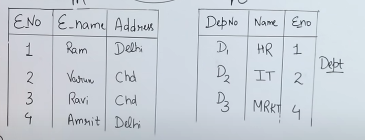
So let's say we have these two tables now :

And we are tasked with this :

This might look similar to Natural Join, but there is a key difference between Natural Join and Equi Join: In Natural Join we check for equality between the common attributes of the two tables, but in Equi Join we can also check for equality among other, non-common attributes of the two tables.

So starting off, we would have our Natural Join query as :

SELECT E_Name from emp, dept WHERE emp.E_Name = dept.E_Name

and this is the point the query becomes an Equi Join query. We check whether two non-common attributes, i.e Address from emp table and Location from dept table are equal or not.

So:

SELECT E_Name from emp, dept WHERE emp.E_Name = dept.E_Name AND emp.Address = dept.Location

Now this is an Equi Join query.

So the final output table for this query will be :

Note that although employee 4 Ravi had the address as Delhi but his department location was in Patna so there was a mismatch in the second parameter of the condition and thus he was not included in the output table.

5. Left-Outer Join

https://www.youtube.com/watch?v=unxn0KnzBzk&list=PLxCzCOWd7aiFAN6I8CuViBuCdJgiOkT2Y&index=43

So let's say we again have these two tables here

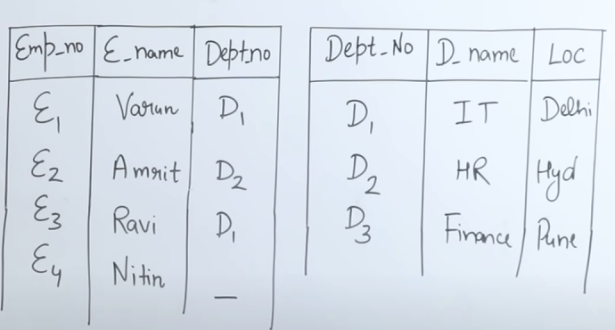
Left-Outer Join returns the matching rows and the rows which are only present in the left table, but not in the right table.

We can clear this concept with the help of a Venn Diagram.

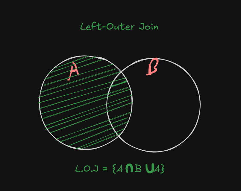
So Left-outer-Join works on top of the standard natural join query.

So let's say if we wanted to perform a Left-Outer Join on these two tables, it would be in this way.

SELECT emp_no, e_name, d_name, loc from emp LEFT OUTER JOIN dept on (emp.dept_no = dept.dept_no)

This time dept_no is the common attribute in the two tables so we go for those. The part after on is the natural join part.

Now this query will return us a table :

The first three rows were the matching rows as a result of the Natural Join operation.

But since the the actual operation is a Left-Outer Join, the fourth row is added to the table as well since it belongs to the left table despite there being no match for employee 4 in the right table.

6. Right-Outer Join

The reverse of Left-Outer Join.

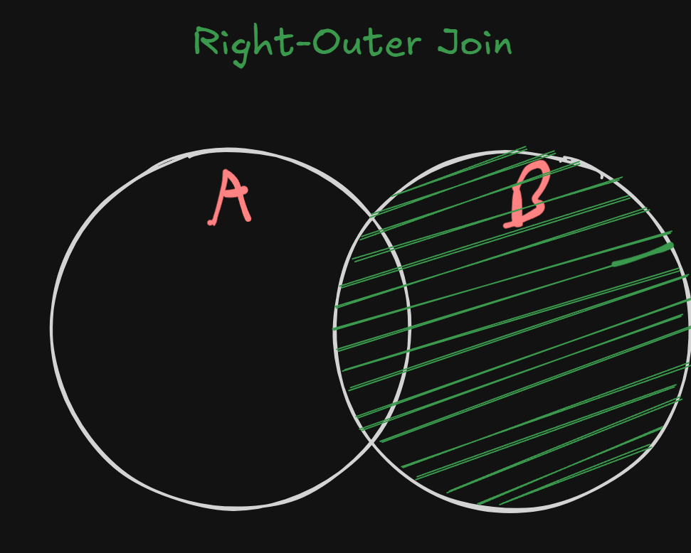
Queries are the same as well, we just replace left outer join with right outer join.

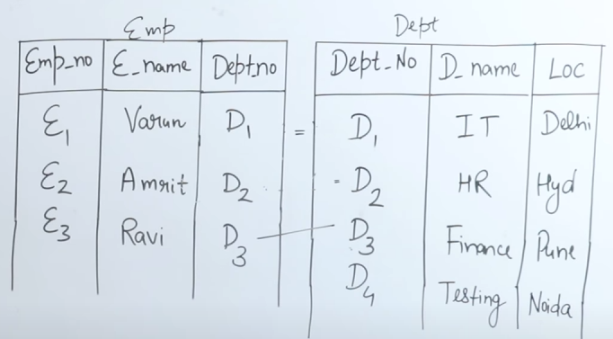
SELECT emp_no, e_name, d_name, loc from emp RIGHT OUTER JOIN dept on (emp.dept_no = dept.dept_no)

So output table will be:

Note that this output table contains the department name of Testing and it's location Noida since it's on the right table.

. Query Optimization Techniques

1. Cost-Based Optimization

• Overview:
  The optimizer uses statistics (e.g., table sizes, index selectivity) to estimate the cost of various execution plans.
• Example Metrics:
  • Estimated I/O operations.
  • CPU costs.
  • Memory usage.

2. Heuristic-Based Rewriting

• Common Heuristics:
  • Push Selections Down:
    Apply selection operations as early as possible to reduce the size of intermediate results.
  • Join Order:
    Reorder join operations to start with the most selective joins (i.e., those that produce the smallest intermediate result).
  • Combine Projections:
    Remove unneeded columns early to reduce data volume.

3. Example Scenario

Consider a query that joins Orders and Customers on customer_id:

• Plan 1:
  Use a nested loop join with Orders as the outer relation. If Orders is very large and Customers is small with an index on customer_id, an Index Nested Loop Join might be optimal.

• Plan 2:
  Use a hash join if both relations are large and no suitable indexes exist. The optimizer will build a hash table on the smaller relation (say, Customers) and then scan Orders.

• Plan 3:
  If both tables are pre-sorted on customer_id, a merge join could be highly efficient.

The optimizer estimates the cost for each plan and selects the one with the lowest estimated cost.