Module 3 -- Storage Strategies -- DBMS
Index
Indices
🔹 What are Indices in DBMS?
https://www.youtube.com/watch?v=E--yzX05_k8&list=PLxCzCOWd7aiFAN6I8CuViBuCdJgiOkT2Y&index=94
An index in a database is a data structure that improves the speed of data retrieval operations on a database table at the cost of additional writes and storage to maintain the index.
In simple terms, indexing reduces the number of blocks to be called from storage during the processing of a query, thus reducing the time taken for the query to execute.
Think of it like the index in a book—instead of flipping through every page, you can directly go to the page number associated with a topic. Similarly, an index in a database lets the DBMS quickly locate data without scanning the entire table.
🔹 Why Use Indexing?
- Fast search: Speeds up
SELECTqueries significantly. - Efficient sorting: Useful for
ORDER BY,GROUP BYoperations. - Quick access to rows with specific column values.
- Reduces CPU and I/O usage.
🔹 How Do Indices Work?
Internally, an index creates a mapping between key values and the location (address or row ID) of the data in the table.
For example:
Employee Table
+----+--------+-------+
| ID | Name   | Dept  |
+----+--------+-------+
| 1  | Alice  | HR    |
| 2  | Bob    | IT    |
| 3  | Carol  | IT    |
+----+--------+-------+

Index on Dept:
{ "HR" -> row 1, "IT" -> rows 2 and 3 }
🔹 Types of Indices
https://www.youtube.com/watch?v=vjrHiaIfOl8&list=PLxCzCOWd7aiFAN6I8CuViBuCdJgiOkT2Y&index=97
https://www.youtube.com/watch?v=4E-MGnjMhRw&list=PLxCzCOWd7aiFAN6I8CuViBuCdJgiOkT2Y&index=98
https://www.youtube.com/watch?v=UpJ9ICmzaAM&list=PLxCzCOWd7aiFAN6I8CuViBuCdJgiOkT2Y&index=99
https://www.youtube.com/watch?v=Ua08uVgsk4k&list=PLxCzCOWd7aiFAN6I8CuViBuCdJgiOkT2Y&index=100
-
Primary Index
- Built on a primary key.
- One per table.
- Unique and sorted.
- Example: Index on
Employee.ID.
-
Secondary Index
- Built on non-primary attributes (e.g.,
Dept). - Can have duplicates.
- Helps in searching non-key attributes.
- Built on non-primary attributes (e.g.,
-
Clustered Index
- Alters the physical order of the data in the table to match the index.
- Only one per table.
- Faster for range queries.
- Used for sorting large data efficiently.
-
Non-clustered Index
- Logical ordering of data.
- Contains pointers to the actual data location.
- Can be multiple per table.
-
Composite Index
- Index on multiple columns (e.g.,
Name, Dept). - Helps if queries filter by more than one column.
- Index on multiple columns (e.g.,
🔹 When to Use Indices
Use indexing:
- When querying large tables frequently.
- On columns used in WHERE, JOIN, GROUP BY, ORDER BY.
- On columns with high selectivity (many unique values).
Avoid indexing:
- On columns with few distinct values (e.g.,
Gender). - On tables with frequent writes/updates (index maintenance overhead).
- If the table is small (full scan is already fast).
🔹 Cost of Indexing
- Extra storage needed.
- Slower insert/update/delete operations.
- Index must be maintained when data changes.
A numerical example to further clear the understanding of Indices.
https://www.youtube.com/watch?v=P24LAhp-ap8&list=PLxCzCOWd7aiFAN6I8CuViBuCdJgiOkT2Y&index=95 (part 1)
https://www.youtube.com/watch?v=s_S_MpLoDEM&list=PLxCzCOWd7aiFAN6I8CuViBuCdJgiOkT2Y&index=96 (part 2)
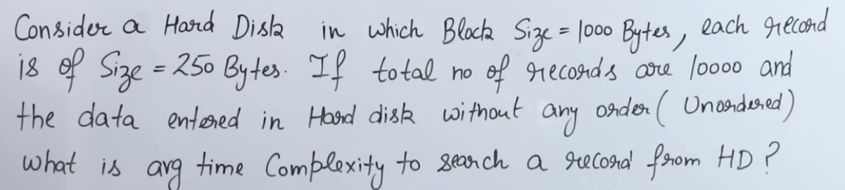
So let's say we have this setup.
Each block in the HDD can hold 1000bytes and each record is of size 250 bytes.
So, number of records per block = 4.
Now if the total number of records were 10,000 (unordered), meaning the records could be scattered on the HDD in a random order.
Total number of blocks required = 2500.
Now let's say we had a query to execute:
SELECT * FROM STUDENTS WHERE ROLL = 345;
How long do you think would that query take to complete, without indices?
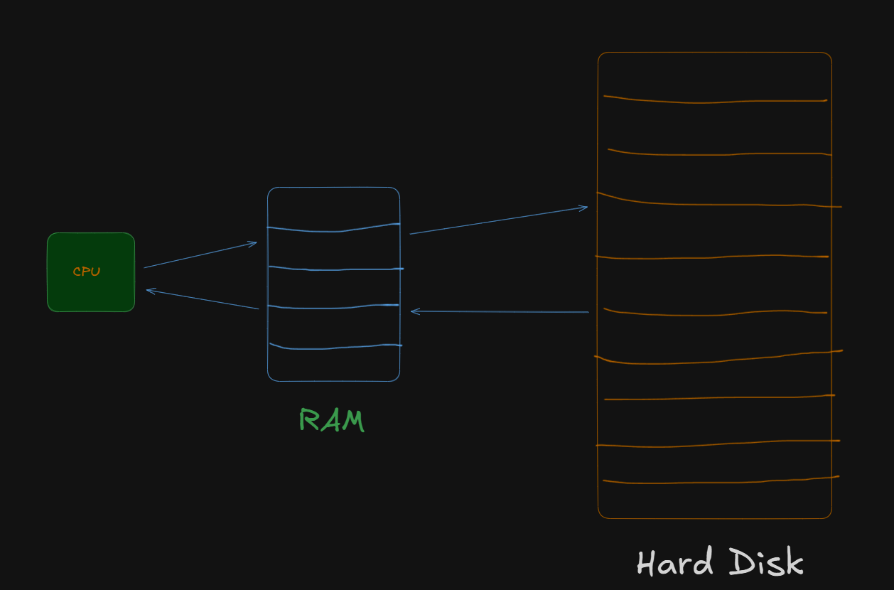
If each block takes a total of 4ms to get processed in the ram and
If we are focusing on the average time complexity then this would be :
And number of blocks needed to scan in average time complexity would 1250.
So, if the worst case scenario is scanning all 2500 blocks, that is the data is present on the 2500th block, then it would N.
Best case scenario would be on the first block, so 1.
So average case time complexity would be:
If the data was ordered then it would be:
12 blocks would be needed to scan and time taken would be 48ms.
Using Indices.
Now using Indices we can get that in an even lower amount of time and lesser amount of blocks.
If the question were to modified as to find the time complexity to search a record from index table if the size of an index table entry is equal to 20 bytes.
Now there can be two types of indexing based on whether the data is ordered or unordered.
For unordered data, we have dense indexing. This means that each block in the index table will have the same number of entries as the ones in the HDD.
For ordered data we have sparse indexing. This means that each block will contain only the page number of the corresponding block in the HDD.
The difference can be spotted in this way:
For 1000 records, a single block of 20 bytes can hold 50 records.
In sparse indexing this would get us =
Which means that the entirety of 1000 records can be fitted in just 50 blocks, as compared to 2500 blocks on the HDD.
This makes the search time much lesser since the time complexity now becomes :
And plus 1 since after searching these 6 records we will get a page number pointing to the desired block on HDD, where we need to perform a search for the desired data value.
For dense indexing we can't use the page index so we need to fit all 10,000 records, we would need 200 blocks for that.
That would result in the time complexity of
And that's why indexing is really helpful in reducing query processing time, specifically searches.
B - Tree
https://www.youtube.com/watch?v=KcApkM5WYGw&list=PLxCzCOWd7aiFAN6I8CuViBuCdJgiOkT2Y&index=108
🌳 What is a B-Tree?
A B-Tree is a self-balancing tree data structure that maintains sorted data and allows searching, insertion, and deletion in logarithmic time.
- It's mainly used in database systems and file systems.
- B-Trees are especially good for disk-based storage (i.e., secondary memory like hard drives).
- It's often used for multilevel indexing.
🧠 Why do we need B-Trees?
-
When data is stored in secondary memory, we want fast ways to search through it.
-
Instead of scanning all records, we build indexes that contain:
- A key (e.g., roll number, student ID)
- A pointer (to the full record in memory)
-
Indexes can get large too, so we make indexes of indexes → multilevel indexing.
-
But multilevel indexing can become slow or hard to update (insert/delete = pain).
-
So, we use a tree structure to organize and balance the index → That’s where B-Trees come in.
📐 B-Tree Terminology
Let’s go over the components the video describes:
1. Nodes
Like all trees, B-trees have:
- Root node – the top node
- Intermediate nodes – internal nodes in the middle
- Leaf nodes – nodes at the bottom
Important: A B-Tree is always balanced, which means all leaf nodes are at the same level.
2. Keys
- Keys are values on which we search (e.g., roll number, name ID, etc.).
- Each node can contain multiple keys, not just one (unlike binary trees).
- The keys are always sorted in increasing order within a node.
3. Record Pointers
- For each key, there's a record pointer → it points to the actual data in secondary memory.
4. Block Pointers (Tree Pointers)
- These point to child nodes (other nodes in the tree).
- Number of children = number of block pointers.
🔢 Order of B-Tree (denoted as P)
This is very important, as it defines:
- Max children = P
- Max keys = P − 1
- Min children = ⌈P/2⌉ (except for root)
- Min keys = ⌈P/2⌉ − 1
Example:
Let’s say order P = 4 (which is common in questions):
| Component | Value |
|---|---|
| Max children | 4 |
| Max keys | 3 |
| Min children (non-root) | 2 (ceil(4/2)) |
| Min keys (non-root) | 1 (ceil(4/2) - 1) |
| Block pointers per node | = number of children (up to P) |
| Record pointers | = number of keys (up to P − 1) |
Finding the Order of a B-Tree
https://www.youtube.com/watch?v=yGSHbjA4w0o&list=PLxCzCOWd7aiFAN6I8CuViBuCdJgiOkT2Y&index=103
🧱 Structure of a Node
For order P = 4, a typical node can look like:
| K1 | K2 | K3 |
| R1 | R2 | R3 |  ← Record Pointers (point to actual data)
| C1 | C2 | C3 | C4 | ← Block Pointers (to child nodes)
- K1, K2, K3 are keys
- R1, R2, R3 are record pointers
- C1 to C4 are child pointers (aka block/tree pointers)
⚙️ Insertion and Search
- Always maintain sorted order of keys in a node.
- Follows a binary-search-like logic inside nodes.
- If a node becomes overfull, it splits and promotes a key to the parent (this keeps the tree balanced).
Insertion in a B-Tree
https://www.youtube.com/watch?v=YUtUNlLNB5c&list=PLxCzCOWd7aiFAN6I8CuViBuCdJgiOkT2Y&index=102
🧠 Quick Refresher: What is a B-Tree of Order m?
- Each node can have at most
m - 1keys. - Each node can have at most
mchildren. - All leaves appear at the same level.
- The keys within a node are kept sorted.
- Every internal node (except root) must have at least ceil(m/2) - 1 keys.
For order 4 (m = 4):
- Max keys per node = 3 (
m - 1) - Min keys per node (except root) = 1 (
ceil(4/2) - 1 = 2 - 1 = 1) - Max children per node = 4
🎯 Insertion Process in a B-Tree
Let’s say we are inserting the values:
1, 2, 3, 4, 5, 6, 7, 8, 9, 10 into a B-tree of order 4
🔢 Step-by-Step Insertion Walkthrough
Insert 1, 2, 3
- Start with a single node (the root).
- Since max keys per node is 3, you can insert
1, 2, 3directly, in sorted order.
Insert 4
-
Now the node has
[1, 2, 3]. Adding4causes overflow. -
When a node overflows (i.e., wants to store more than
m - 1keys), we:-
Find the median key. Here,
[1, 2, 3, 4]→ median =2(choosing the left median).The process of calculating the median is
We consider the total number of keys including the key which overfills the node.
-
Split the node into two:
- Left child:
[1] - Right child:
[3, 4] - Median
2goes up and becomes the new root.
- Left child:
-
✅ Resulting structure:
         [2]
        /   \
     [1]   [3,4]
Insert 5
- Compare 5 with root
2→ go right to[3, 4]. - Insert
5→ becomes[3, 4, 5](still within limit).
Insert 6
-
Inserting
6into[3, 4, 5]causes overflow. -
Keys =
[3, 4, 5, 6]→ median =4- Left child:
[3] - Right child:
[5, 6] 4is pushed up to the root.
- Left child:
✅ Now root has two keys:
        [2, 4]
       /  |   \
    [1] [3] [5,6]
Insert 7
- Compare with root: 7 > 4 → go right to
[5,6] - Insert 7 → becomes
[5, 6, 7](ok)
Insert 8
-
Insert 8 into
[5, 6, 7]→ overflow again. -
Keys =
[5, 6, 7, 8]→ median =6- Split:
- Left:
[5] - Right:
[7, 8] - Median
6goes up
- Left:
- Split:
Root [2, 4] can accept one more key → becomes [2, 4, 6]
          [2, 4, 6]
        /    |    | \
     [1]   [3]  [5]  [7,8]
Insert 9
- 9 > 6 → go to rightmost node →
[7, 8] - Insert 9 → becomes
[7, 8, 9](ok)
Insert 10
- Add 10 to
[7, 8, 9]→ overflow - Keys =
[7, 8, 9, 10]→ median =8- Left:
[7] - Right:
[9, 10] 8goes up
- Left:
But root [2, 4, 6] is already full, so we need to:
-
Split root:
- Median of
[2, 4, 6, 8]=4 - Left:
[2] - Right:
[6, 8] 4becomes the new root
- Median of
✅ Final structure:
            [4]
        /      \
     [2]         [6, 8]
   /    \        /   | \
[1]   [3]   [5] [7] [9,10]
🧩 Key Concepts to Remember
| Concept | Explanation |
|---|---|
| Order (m) | Max children per node |
| Max keys per node | m - 1 |
| Min keys per node | ceil(m/2) - 1 |
| Overflow | When a node gets more than m - 1 keys |
| Splitting | Happens on overflow → median key goes up, node splits into two |
| Promotion | When a median goes to the parent (may cause cascading splits if full) |
| Sorted Insertions | B-tree maintains sorted order and binary-search-like path finding |
| Balanced Tree | All leaves are at the same level (ensures balanced height for fast access) |
🧪 Why Balanced?
A balanced tree means:
- All paths from root to leaves are of the same length.
- Ensures predictable and efficient performance for searching, inserting, and deleting.
B+ Trees
This is not directly present in our syllabus but is a good reference point.
🌳 What is a B+ Tree?
A B+ Tree is a self-balancing tree data structure that maintains sorted data and allows search, insert, delete, and range queries in logarithmic time.
✅ It’s an extension of the B-tree, optimized for disk-based storage systems (like databases and file systems).
📦 Why B+ Trees in Databases?
Databases need:
- Efficient search and range queries
- Balanced access times
- Minimized disk I/O
The B+ Tree handles these perfectly by:
- Keeping all actual data in the leaf nodes.
- Keeping index/search keys in internal nodes.
- Being shallow in height, so traversals require fewer disk reads.
🧠 Structure of a B+ Tree
-
Internal Nodes:
- Store only keys, not actual data.
- Guide the search path.
-
Leaf Nodes:
- Store data records (or pointers to them).
- Are linked in a singly/doubly linked list for efficient range queries.
-
Order (d):
- Determines the maximum number of children a node can have.
- Each internal node can have at most
2dchildren and at leastd.
🌿 Example Structure (Order d = 2):
        [10 | 20]
       /    |    \
      /     |     \
 [1 5 8] [11 14 18] [21 23 30]   <- leaf nodes (data)
- Root contains keys: 10, 20.
- Internal structure routes you to the right leaf.
- Leaf nodes hold actual data and are linked.
🔎 Searching in B+ Tree
- Start at the root.
- Follow the correct child based on key comparisons.
- Reach a leaf node, then scan for the exact key.
- Time complexity: O(log n).
➕ Insertion in B+ Tree
- Insert into correct leaf node.
- If the node overflows, split it.
- Promote the middle key to the parent node.
- Repeat upward if needed (may grow height).
Example:
Before:
Leaf: [10, 20]
Insert 30 → becomes [10, 20, 30] → Overflow → Split:
- Leaves:
[10], [20, 30] - Internal:
[20]
🔁 Differences Between B Tree and B+ Tree
| Feature | B Tree | B+ Tree |
|---|---|---|
| Data location | Internal & leaf nodes | Only in leaf nodes |
| Range queries | Inefficient | Efficient using linked leaves |
| Leaf linkage | Not required | Linked for faster traversal |
| Storage space | Slightly less efficient | Slightly more (due to duplication of keys) |
| Search | Faster for single key | Slightly more steps (due to leaf-only data) |
📈 Advantages of B+ Trees
- Great for range queries (
WHERE age BETWEEN 20 AND 30) - Better use of disk blocks
- Predictable performance due to shallow depth
- Maintains sorted order
📌 Real Use
- Most relational DBMSs (MySQL, PostgreSQL, Oracle) use B+ Trees for indexing (especially clustered indexes).
- Also used in file systems (e.g., NTFS, HFS+).
Hashing
🔐 What is Hashing?
Hashing is a technique to map data of any size to fixed-size values using a hash function. The result of this mapping is called a hash value or hash code, and it helps you store and retrieve data quickly.
Think of it like assigning a locker number (hash code) to every student (data) so that you can find their locker instantly, without searching every locker.
🎯 Objective of Hashing
- Fast Data Retrieval (especially in constant time — O(1) on average)
- Used in databases, caches, compilers, cryptography, etc.
🧮 Hash Table
A hash table is a data structure that uses hashing to store key-value pairs.
- It consists of an array.
- Each index in the array is called a bucket or slot.
- A hash function is used to calculate the index (slot) from a key.
🔄 Hash Function
A hash function h(k) maps a key k to an index in the array.
h(k) = k mod m
Where:
kis the key (like a student roll number)mis the size of the hash table
So if:
k = 123, andm = 10
Then:h(123) = 123 % 10 = 3
So, store the data at index 3.
❗ Collisions in Hashing
A collision happens when two different keys hash to the same index.
Example:
h(123) = 3h(133) = 3
Now both 123 and 133 want to go into index 3 → Collision!
We solve this using Collision Resolution Techniques.
🛠️ Collision Resolution Techniques
1. Open Hashing / Chaining
- Each slot in the hash table points to a linked list (or chain) of values.
- All values that hash to the same index are stored in the list at that index.
Index 3 → [123] → [133]
2. Closed Hashing / Open Addressing
- All elements are stored within the hash table itself (no linked lists).
- If a slot is occupied, it searches for another slot using a probing technique.
a. Linear Probing
- Check the next slot:
h(k), h(k)+1, h(k)+2, ... - Formula:
(h(k) + i) mod m
b. Quadratic Probing
- Uses a quadratic function to jump:
h(k) + i² - Formula:
(h(k) + c₁*i + c₂*i²) mod m
c. Double Hashing
- Uses a second hash function to decide the jump length.
- Formula:
(h1(k) + i*h2(k)) mod m
💡 Load Factor (α)
α = number of elements / size of hash table- It measures how full the hash table is.
- The performance of a hash table depends on load factor.
- Too high → more collisions → slow
- Too low → waste of space
📦 Applications of Hashing
- Database indexing
- Password storage (with cryptographic hashing)
- Symbol tables in compilers
- Caching mechanisms
- Sets and maps in programming languages (e.g., Python's
set,dict, Java’sHashMap)
✅ Summary
| Term | Meaning |
|---|---|
| Hashing | Mapping key to index |
| Hash Function | Converts key to index |
| Hash Table | Array storing data using hash values |
| Collision | Multiple keys map to same index |
| Chaining | Linked list at each slot |
| Linear/Quadratic/Double Probing | Methods to resolve collisions without chaining |
| Load Factor | Measure of how full the table is |