Index

1. Parallel Architectures
2. Parallel Query Processing

Parallel Architectures

https://www.geeksforgeeks.org/design-of-parallel-databases-dbms/

Parallel Architectures in Parallel Database Systems

Parallel database systems leverage multiple processors or machines to execute database operations concurrently, improving performance for large-scale data processing. The architecture defines how these processors, memory, and storage are organized. There are three main types of parallel architectures:

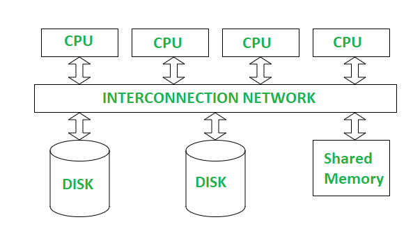
• Shared-Memory Architecture:

  • What It Is: Multiple processors share a single, common memory space and access a shared disk for storage.

  • How It Works: All processors can directly read/write to the same memory, making communication between them fast since they don’t need to send messages over a network.

  • Pros:

    • Fast data sharing and communication between processors due to direct memory access.
    • Simpler to program since there’s no need to handle network communication.

  • Cons:

    • Limited scalability—adding more processors leads to memory contention (bottleneck when multiple processors try to access the same memory simultaneously).
    • Not ideal for very large systems due to this bottleneck.

  • Example: A small-scale parallel database system with 4 processors sharing 64GB of RAM to process queries on a single database stored on a shared disk.

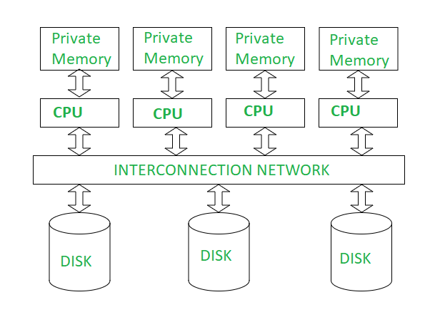
• Shared-Disk Architecture:

  • What It Is: Each processor has its own private memory, but all processors share a common disk for storage.

  • How It Works: Processors communicate via a high-speed interconnect to access the shared disk. Each processor works independently with its own memory but retrieves data from the same disk.

  • Pros:

    • Better scalability than shared-memory since memory contention is avoided (each processor has its own memory).
    • Easier to manage data consistency since all processors access the same disk.

  • Cons:

    • Disk access can become a bottleneck, especially with many processors trying to read/write simultaneously.
    • Requires a fast interconnect to minimize latency when accessing the disk.

  • Example: A system with 10 processors, each with its own 16GB of RAM, accessing a shared SAN (Storage Area Network) disk to process a large dataset.

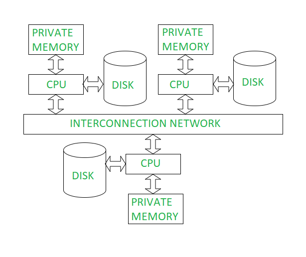
• Shared-Nothing Architecture:

  • What It Is: Each processor has its own private memory and disk, with no shared resources between processors.

  • How It Works: Processors (or nodes) communicate over a network to exchange data or coordinate tasks. Data is partitioned across the nodes, and each node processes its local data independently.

  • Pros:

    • Highly scalable—adding more nodes increases both processing power and storage capacity without contention.
    • Ideal for distributed systems and large-scale databases (e.g., modern DDBSs like Google BigQuery or Apache Cassandra).

  • Cons:

    • Higher communication overhead since nodes must exchange data over a network, which can be slower than shared-memory access.
    • More complex to manage due to data partitioning and network coordination.

  • Example: A cluster of 20 nodes, each with its own CPU, 32GB RAM, and 1TB disk, storing a fragment of a customer database. Nodes communicate over a high-speed network to process a distributed query.

Key Considerations

• Scalability vs. Complexity: Shared-memory is the least scalable but simplest to manage, while shared-nothing is the most scalable but requires careful data partitioning and network management. Shared-disk lies in the middle.
• Performance: Shared-memory offers the best performance for small systems due to fast communication, but shared-nothing shines for large-scale systems where scalability is critical.
• Use in DDBSs: Most modern distributed databases (e.g., Snowflake, Amazon Redshift) use shared-nothing architectures because they align well with distributed systems, allowing massive scalability across many nodes.

Parallel Query Processing

(This was covered previously in module 3 pdf)

https://www.geeksforgeeks.org/parallelism-in-query-in-dbms/

Parallel Query Processing in Parallel Database Systems

Parallel query processing is the technique of dividing a database query into smaller tasks that can be executed concurrently across multiple processors or nodes, significantly speeding up query execution. This is a key feature of parallel database systems, leveraging the architectures we discussed (shared-memory, shared-disk, shared-nothing). Let’s break it down:

• Data Partitioning(Same as fragmentation):

  • What It Is: Splitting the database into smaller fragments (partitions) that can be processed independently by different processors or nodes.

  • How It Works:

    • Horizontal Partitioning: Rows of a table are divided across nodes. For example, a customer table might be split so Node 1 stores customers with IDs 1–1000, Node 2 stores IDs 1001–2000, etc.

    • Vertical Partitioning: Columns of a table are split across nodes (less common in parallel query processing).

    • Hybrid Partitioning: Combines both horizontal and vertical partitioning for more complex scenarios.

  • Purpose: Allows each processor to work on its own subset of data, reducing the workload per processor and enabling parallelism.

  • Example: In a shared-nothing architecture, a 1TB sales table is horizontally partitioned across 10 nodes, with each node storing 100GB. A query to calculate total sales can be executed on all nodes simultaneously, with each node processing its 100GB chunk.

Hash Partitioning in Parallel Query Processing

Hash partitioning is a data partitioning technique used in parallel query processing to distribute data across multiple nodes or processors, enabling parallel execution of queries. It’s particularly effective in shared-nothing architectures, where each node processes its own subset of data independently.

• What It Is:
  Hash partitioning uses a hash function to assign data records to different partitions based on a specific attribute (called the partitioning key). The goal is to distribute data evenly across nodes to balance the workload.

• How It Works:

  • A hash function (e.g., modulo operation) is applied to the partitioning key of each record.
  • The result of the hash function determines which node or partition the record is assigned to.
  • Formula: If there are $N$ nodes, a record with partitioning key $K$ is assigned to node $hash(K)\mathrm{mod}N$
  • The hash function ensures that records with the same key value are always assigned to the same node (useful for operations like joins).

• Example:

  • Consider a customer table with a “CustomerID” as the partitioning key, and 4 nodes (Node 0 to Node 3).
  • A hash function is applied: $hash(CustomerID)\mathrm{mod}4$
  • If $CustomerID=123$, and $hash(123)=15$, then $15\mathrm{mod}4=3$, so the record goes to Node 3.
  • If $CustomerID=456$, and $hash(456)=10$, then $10\mathrm{mod}4=2$ , so the record goes to Node 2.
  • A query like “SELECT * FROM customers WHERE CustomerID = 123” is routed directly to Node 3, which processes it locally.

• Pros:

  • Even Distribution: The hash function typically distributes data uniformly across nodes, avoiding workload imbalances (unless there’s significant skew in the key values).
  • Efficient Lookups: Queries that filter on the partitioning key (e.g., equality conditions like “CustomerID = 123”) can be routed directly to the relevant node, minimizing data movement.
  • Good for Joins: If two tables are partitioned on the same key using the same hash function, join operations can be performed locally on each node without shuffling data.

• Cons:

  • Skew Issues: If the partitioning key has many duplicate values (e.g., a “Gender” column with only “M” and “F”), the hash function may assign most records to a few nodes, causing data skew and uneven workloads.
  • Range Queries Inefficient: Range queries (e.g., “SELECT * FROM customers WHERE CustomerID BETWEEN 100 AND 200”) may need to access all nodes, as the hash function scatters values non-sequentially.
  • Rehashing Overhead: Adding or removing nodes requires rehashing and redistributing all data, which can be costly.

• Use Case:
  Hash partitioning is ideal for workloads with many equality-based queries or joins, such as in a retail database where you frequently query by “OrderID” or join orders and customers tables on “CustomerID”.

Range Partitioning in Parallel Query Processing

Range partitioning is another data partitioning technique used in parallel query processing to distribute data across nodes or processors, enabling parallel execution. Unlike hash partitioning, which uses a hash function, range partitioning divides data based on predefined ranges of a partitioning key, making it particularly suited for certain types of queries.

• What It Is:
  Range partitioning assigns records to nodes based on whether the value of a partitioning key falls within a specific range. Each node is responsible for a distinct, non-overlapping range of values.

• How It Works:

  • The partitioning key (e.g., a numeric or date column) is divided into ranges.
  • Each node is assigned a specific range, and records are placed on the node whose range includes the record’s key value.
  • The ranges are typically defined to balance the data distribution across nodes, though this depends on the data’s distribution.
  • Example Setup:
    • Partitioning key: “OrderDate” (a date column).
    • 4 nodes:
      • Node 0: OrderDate < 2020-01-01
      • Node 1: 2020-01-01 ≤ OrderDate < 2021-01-01
      • Node 2: 2021-01-01 ≤ OrderDate < 2022-01-01
      • Node 3: OrderDate ≥ 2022-01-01

• Example:

  • A sales table with an OrderDate column is range-partitioned across 4 nodes as above.
  • A record with OrderDate = “2021-06-15” goes to Node 2 (since it falls in the range 2021-01-01 to 2021-12-31).
  • A query like “SELECT * FROM sales WHERE OrderDate BETWEEN 2021-01-01 AND 2021-12-31” is routed directly to Node 2, which processes it locally.
  • A query like “SELECT * FROM sales WHERE OrderDate < 2021-01-01” involves Nodes 0 and 1 but skips Nodes 2 and 3, reducing the workload.

• Pros:

  • Efficient Range Queries: Range partitioning excels for range-based queries (e.g., “WHERE OrderDate BETWEEN X AND Y”) because only the nodes with the relevant ranges need to be accessed, minimizing data scanning.
  • Sequential Access: If the partitioning key is ordered (e.g., dates or numbers), data within each node is also ordered, which can speed up operations like sorting or range scans.
  • Predictable Distribution: You can define ranges to control data placement, which can be useful for workloads with known access patterns.

• Cons:

  • Data Skew: If the data distribution is uneven, some ranges may have more records than others, leading to workload imbalances.
    • Example: If most sales are from 2022 onwards, Node 3 will be overloaded while Nodes 0–2 are underutilized.
  • Inefficient for Equality Queries: Unlike hash partitioning, equality queries (e.g., “WHERE OrderDate = ‘2021-06-15’”) still require identifying the correct range, which might be less direct than a hash lookup.
  • Range Adjustments: Adding or removing nodes requires redefining ranges and redistributing data, which can be complex and time-consuming.

• Use Case:
  Range partitioning is ideal for workloads with frequent range queries or time-based data, such as in a financial database where you often query transactions by date ranges (e.g., “all transactions in Q1 2024”). It’s also common in data warehousing systems like Amazon Redshift or Snowflake for handling time-series data.

Schema Partitioning in Parallel Query Processing

Schema partitioning (sometimes referred to as vertical partitioning in the context of parallel query processing) involves dividing a database table based on its schema—specifically, by splitting the columns (attributes) of the table across different nodes or processors. This is less common than horizontal partitioning methods like hash or range partitioning but can be useful in specific scenarios.

• What It Is:
  Schema partitioning splits a table vertically by distributing its columns across multiple nodes, rather than splitting rows. Each node stores a subset of the table’s attributes for all rows, along with a common key to link the data back together when needed.

• How It Works:

  • The table’s columns are divided into groups, and each group is assigned to a node.

  • A primary key (or a unique identifier) is typically stored on all nodes to allow records to be joined back together during query execution.

  • When a query is executed, nodes process their subset of columns in parallel, and the results are combined using the common key.

  • Example Setup:

    • Table: Employees (EmpID, Name, Department, Salary, HireDate)
    • 3 nodes:
      • Node 0: Stores EmpID, Name
      • Node 1: Stores EmpID, Department, Salary
      • Node 2: Stores EmpID, HireDate
    • EmpID is the common key stored on all nodes to link the data.

• Example:

  • Using the Employees table above, a record with EmpID = 101, Name = "Alice", Department = "HR", Salary = 60000, HireDate = "2020-01-15" is split as:

    • Node 0: (101, "Alice")
    • Node 1: (101, "HR", 60000)
    • Node 2: (101, "2020-01-15")

  • A query like SELECT Name, Salary FROM Employees WHERE EmpID = 101 requires:

    • Node 0 to provide the Name ("Alice").
    • Node 1 to provide the Salary (60000).
    • The results are joined using EmpID = 101 to return ("Alice", 60000).

  • A query that only needs HireDate (e.g., SELECT HireDate FROM Employees) can be handled entirely by Node 2, avoiding the other nodes.

• Pros:

  • Efficient for Column-Specific Queries: If a query only accesses a subset of columns, it can be processed by fewer nodes, reducing I/O and processing overhead.

    • Example: A query needing only HireDate doesn’t need to involve Nodes 0 or 1.

  • Reduced Data Transfer: Nodes only send the columns they manage, which can minimize network traffic in a shared-nothing architecture.

  • I/O Optimization: Since each node deals with fewer columns, it may need to read less data from disk, improving performance for column-heavy tables.

• Cons:

  • Join Overhead: Queries that need columns from multiple nodes require joining the data using the common key, which can be expensive, especially if the join involves a large number of records.

  • Complexity: Managing schema partitioning is more complex than row-based partitioning, as the system must track which columns are on which nodes and handle joins efficiently.

  • Limited Use Cases: Schema partitioning is less common in parallel query processing because most queries in DDBSs operate on rows, not columns. It’s more useful in column-oriented databases (e.g., Vertica or Google BigQuery).

• Use Case:
  Schema partitioning is ideal for analytical workloads where queries often access a small subset of columns, such as in data warehousing. For example, a financial database might frequently query only the TransactionID and Amount columns, so storing these together on one node can optimize performance. It’s also useful in systems where storage constraints require splitting wide tables (tables with many columns) across nodes.

Round-Robin Partitioning in Parallel Query Processing

Round-robin partitioning is a simple data partitioning technique used in parallel query processing to distribute data across nodes or processors. Unlike hash or range partitioning, which use a partitioning key to determine data placement, round-robin partitioning distributes data in a cyclic, sequential manner, focusing on achieving an even distribution.

• What It Is:
  Round-robin partitioning assigns records to nodes in a circular order, one record at a time, without considering any specific attribute of the data. The goal is to ensure an equal distribution of records across nodes, regardless of the data values.

• How It Works:

  • Records are distributed to nodes in a sequential, rotating fashion: the first record goes to Node 1, the second to Node 2, the third to Node 3, and so on, looping back to Node 1 after reaching the last node.
  • No partitioning key is used—the placement is purely based on the order of insertion.
  • Example Setup:
    • 4 nodes: Node 0, Node 1, Node 2, Node 3.
    • A table with 8 records is partitioned:
      • Record 1 → Node 0
      • Record 2 → Node 1
      • Record 3 → Node 2
      • Record 4 → Node 3
      • Record 5 → Node 0
      • Record 6 → Node 1
      • Record 7 → Node 2
      • Record 8 → Node 3

• Example:

  • A sales table with 8 records (e.g., SaleID 1 to 8) is distributed across 4 nodes using round-robin partitioning, as shown above.
  • A query like SELECT * FROM sales WHERE SaleID = 5 knows that SaleID 5 is on Node 0 (since 5 mod 4 = 1, but counting nodes as 0 to 3, it cycles as shown).
  • A query like SELECT SUM(Amount) FROM sales can be executed in parallel, with each node summing its local records (e.g., Node 0 sums records 1 and 5, Node 1 sums records 2 and 6, etc.), and the results are combined.

• Pros:

  • Guaranteed Even Distribution: Since records are assigned in a cyclic manner, each node gets roughly the same number of records, ensuring balanced workloads.
    • Example: With 1000 records and 4 nodes, each node gets exactly 250 records.
  • Simple to Implement: No need for a partitioning key or complex logic—just distribute records in order.
  • Good for Sequential Workloads: Works well for queries that scan the entire table (e.g., aggregations like SUM or COUNT), as all nodes can process their equal share in parallel.

• Cons:

  • Inefficient for Key-Based Queries: Since placement is not based on data values, queries that filter on a specific attribute (e.g., WHERE SaleID = 5 or WHERE OrderDate > '2023-01-01') may need to scan all nodes, as there’s no guarantee that related records are co-located.
  • Joins Are Expensive: If two tables need to be joined on a key, round-robin partitioning offers no locality—data must be shuffled across nodes, increasing network overhead.
  • No Semantic Grouping: Unlike hash or range partitioning, round-robin doesn’t group related data together, which can hurt performance for selective queries.

• Use Case:
  Round-robin partitioning is ideal for workloads where data distribution needs to be perfectly balanced and queries are mostly full-table scans or aggregations, such as in a data warehouse running SELECT AVG(Salary) FROM employees. It’s less suitable for transactional systems with frequent key-based lookups or joins. Systems like Apache Hive or Spark sometimes use round-robin partitioning for initial data distribution when the access pattern is unknown.

Quick Recap of Partitioning Types

• Hash Partitioning: Uses a hash function on a key to distribute data; good for equality queries and joins.
• Range Partitioning: Divides data into ranges based on a key; great for range queries (e.g., time-based data).
• Schema Partitioning: Splits columns across nodes; useful for column-specific queries but complex for joins.
• Round-Robin Partitioning: Distributes data cyclically; ensures even distribution but inefficient for key-based queries.

• Parallel Execution Strategies:

  • Intra-Operation Parallelism:

    • What It Is: Parallelizing a single operation within a query.
    • How It Works: An operation like a scan, sort, or join is divided into smaller tasks that run concurrently.
    • Example: A query requires scanning a table to find all sales from 2024. If the table is partitioned across 4 nodes, each node scans its partition in parallel, and the results are combined.
    • Benefit: Speeds up individual operations, especially for large datasets.

  • Inter-Operation Parallelism:

    • What It Is: Executing different operations of a query in parallel.
    • How It Works: Operations like filtering, joining, and aggregating can run simultaneously if they’re independent. This often involves pipelining, where the output of one operation feeds directly into the next.
    • Example: A query joins two tables (sales and customers) and then filters for sales above $500. The join operation can run on some nodes while the filter operation runs on others, with data flowing between them in a pipeline.
    • Benefit: Reduces overall query execution time by overlapping operations.

• Query Optimization in Parallel Systems:

  (This was covered previously in module 3 pdf)

  • What It Is: The process of determining the most efficient way to execute a query in a parallel environment.

  • How It Works:

    • Data Locality: The optimizer assigns tasks to nodes where the data resides to minimize data movement across the network (especially in shared-nothing architectures).
    • Load Balancing: Ensures tasks are distributed evenly across nodes to avoid bottlenecks (e.g., one node being overloaded while others are idle).
    • Cost Estimation: The optimizer estimates the cost of different execution plans (e.g., considering CPU, I/O, and network costs) and chooses the best one.

  • Example: A query joins two tables, one stored on Node 1 and the other on Node 2. The optimizer might decide to move the smaller table to Node 1 for the join (to minimize network transfer) and then distribute the join operation across both nodes for parallel processing.

  • Challenges:

    • Network overhead in shared-nothing systems can slow down data movement.
    • Skewed data (e.g., uneven partitioning) can lead to imbalanced workloads.

Key Considerations

• Relation to Architectures:

  • In shared-memory systems, parallel query processing is simpler since all processors can access the same data directly, but scalability is limited.
  • In shared-nothing systems, data partitioning is critical, and network communication must be minimized to maintain performance.

• Performance Gains: Parallel query processing can dramatically reduce query execution time. For example, a query that takes 100 seconds on a single processor might take only 10 seconds on 10 processors (ideally, though real-world factors like overhead reduce this gain).

• Modern Systems: Systems like Snowflake, Google BigQuery, and Apache Spark heavily rely on parallel query processing, using shared-nothing architectures to scale across thousands of nodes.