Unsupervised Learning -- Module 2 -- Machine Learning
Index
- Clustering K-Means and Kernel K-Means
- Kernel K-Means
- Dimensionality Reduction - PCA and Kernel PCA
- Back to PCA then, with an example
- Kernel PCA
- Matrix factorization
- 1. Singular Value Decomposition
- Matrix Completion
- 1. Gradient Descent
- Generative Models
Clustering: K-Means and Kernel K-Means
The K-Means Algorithm
At this point we already know what the K-Means algorithm is, still I will add the content again. If you do not wish to study this, skip ahead to Kernel K-Means
Basic Idea:
Divides n objects into k clusters, where each object belongs to the cluster with the nearest mean (called the centroid).
The K-Means algorithm begins by randomly assigning each data point to a cluster. It then iteratively refines the clusters' centroids until convergence. The refinement process involves calculating the mean of the data points assigned to each cluster and updating the cluster centroids' coordinates accordingly. The algorithm continues to iterate until convergence, meaning the cluster assignments no longer change. K-means clustering aims to minimize the sum of squared distances between each data point and its assigned cluster centroid.
Before we proceed further, let's understand about :
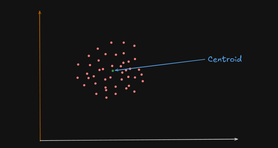
What is a Centroid?
A centroid is the geometric center of a cluster.
Or
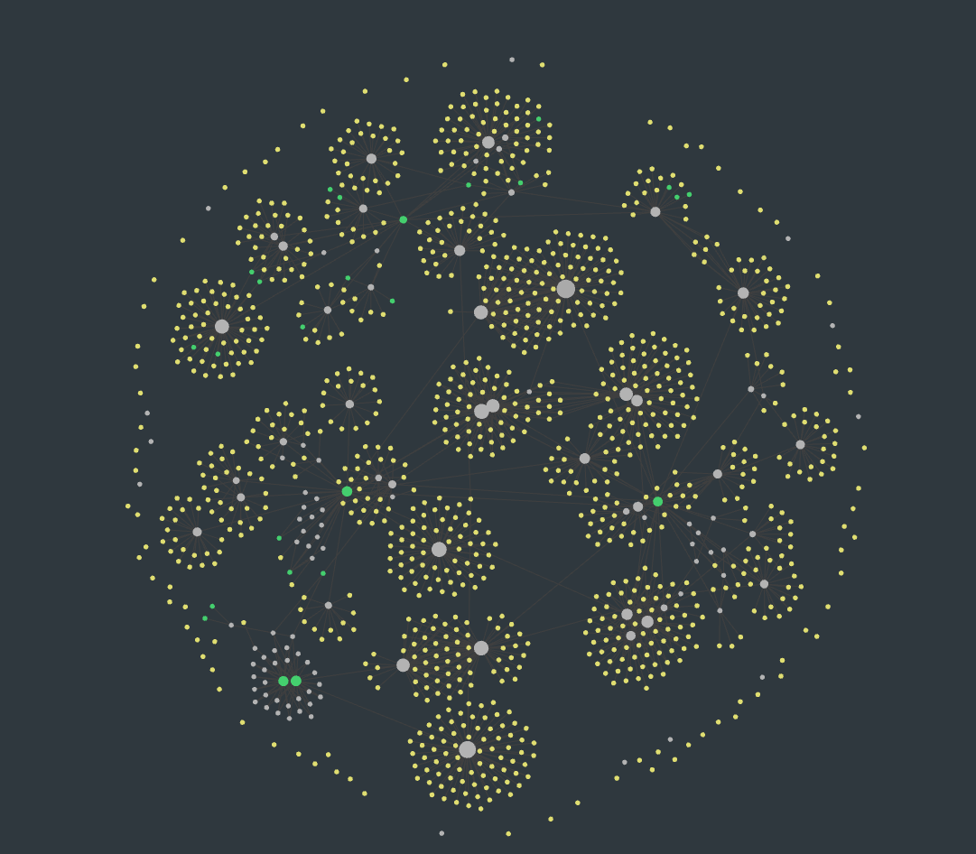
One could say that the centroid of these clusters are the big white circles at the center, and in some cases, the green circles
It’s like the average position of all the points (data samples) assigned to that cluster.
For example :
Let’s say you have a 2D space where each data point is represented by coordinates:
| Point | X | Y |
|---|---|---|
| A | 2 | 4 |
| B | 4 | 6 |
| C | 3 | 5 |
| If these three points belong to a single cluster, the centroid’s coordinates would be calculated like this: |
So the centroid of all these data points is
In higher dimensions(more number of variables), the centroid is still just the mean of each coordinate (feature) across all points in the cluster and the centroid formula scales as follows :
Why Is It Important?
1️⃣ The centroid acts like the "anchor" for a cluster. 2️⃣ During the K-Means algorithm:
- Data points are assigned to the cluster whose centroid is closest.
- Centroids are recalculated based on the new points assigned.
- This process continues until centroids stop changing.
Important:
- The centroid might not be an actual data point.
- It’s just the mathematical center, and sometimes no real data point is located there.
- In contrast, K-Medoids uses real data points as centers, not averages.
So, getting back to K-Means clustering,
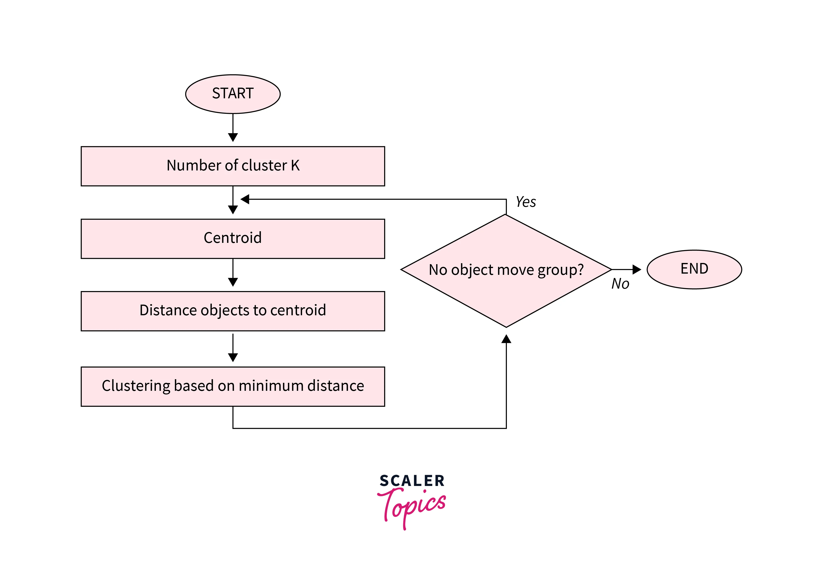
Algorithm of K-Means clustering
- Choose the number of clusters
k. - Randomly choose
kcentroids. - Assign each point to the nearest centroid. (This is done by calculating the distance of a point to all the centroids then assigning that point to the centroid with the lowest distance, thus creating a cluster)
- Re-compute centroids as the mean of all points in the cluster (using the centroid formula).
- Repeat steps 3 & 4 until centroids don’t change (convergence is reached) or a maximum number of iterations is reached.
Advantages of K-Means
Here are some advantages of the K-means clustering algorithm -
- Scalability - K-means is a scalable algorithm that can handle large datasets with high dimensionality. This is because it only requires calculating the distances between data points and their assigned cluster centroids.
- Speed - K-means is a relatively fast algorithm, making it suitable for real-time or near-real-time applications. It can handle datasets with millions of data points and converge to a solution in a few iterations.
- Simplicity - K-means is a simple algorithm to implement and understand. It only requires specifying the number of clusters and the initial centroids, and it iteratively refines the clusters' centroids until convergence.
- Interpretability - K-means provide interpretable results, as the clusters' centroids represent the centre points of the clusters. This makes it easy to interpret and understand the clustering results.
Disadvantages of K-Means
Here are some disadvantages of the K-means clustering algorithm -
-
Curse of dimensionality - K-means is prone to the curse of dimensionality, which refers to the problem of high-dimensional data spaces. In high-dimensional spaces, the distance between any two data points becomes almost the same, making it difficult to differentiate between clusters. (Kernel K-Means will focus on solving this. Similar to how Kernels solve the curse of dimensionality in SVMs)
-
User-defined K - K-means requires the user to specify the number of clusters (K) beforehand. This can be challenging if the user does not have prior knowledge of the data or if the optimal number of clusters is unknown.
-
Non-convex shape clusters - K-means assumes that the clusters are spherical, which means it cannot handle datasets with non-convex shape clusters. In such cases, other clustering algorithms, such as hierarchical clustering or DBSCAN, may be more suitable.
-
Unable to handle noisy data - K-means are sensitive to noisy data or outliers, which can significantly affect the clustering results. Preprocessing techniques, such as outlier detection or noise reduction, may be required to address this issue.
Kernel K-Means
The Problem with Regular K-means
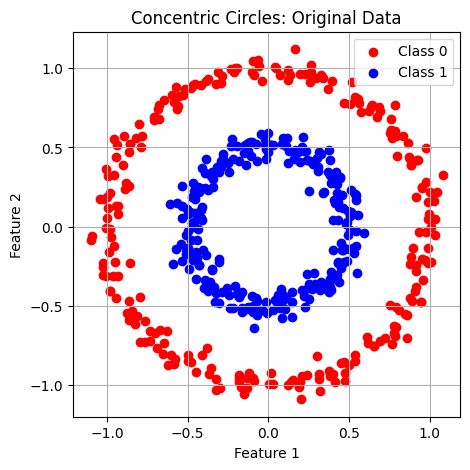
Regular K-means works well when clusters are linearly separable - meaning you can draw straight lines (or hyperplanes) to separate the clusters. However, many real-world datasets have clusters that follow non-linear patterns like:
-
Concentric circles
-
Spiral shapes
-
Interleaved patterns
In these cases, regular K-means fails because it assumes clusters are spherical and separated by linear boundaries.
What is Kernel K-means?
Kernel K-means extends regular K-means to handle non-linear cluster structures by using the kernel trick. Instead of working directly with the original data points, it implicitly maps them to a higher-dimensional feature space where the clusters become linearly separable
The key insight: What looks non-linear in the original space might become linear in a transformed space.
So basically the same kernel trick that happens in SVMs
The Kernel Trick in Clustering
Core Concept
Rather than explicitly transforming data points
This allows us to work in high-dimensional spaces without actually computing the transformation.
Distance Calculation
In kernel K-means, the distance between a data point
(Don't really stress on the equation here.)
Using the kernel trick, this becomes:
Where
(We might need to know this equation)
Common Kernel Functions
1. Polynomial Kernel (General form)
Formula:
- Parameters: degree
, constant - Use case: When clusters have polynomial boundaries
2. Radial Basis Function (RBF/Gaussian) Kernel
Formula:
- Parameter: bandwidth
- Use case: Most versatile; handles complex, smooth cluster shapes
3. Sigmoid Kernel
Formula:
- Parameters:
, constant - Use case: Neural network-inspired clustering
Kernel K-means Algorithm
Here are the step-by-step algorithmic procedures.
At the base it's the same K-Means algorithms with the distance metric swapped out with a different method using a specific Kernel.
Input: Dataset
- Initialize: Randomly assign each data point to one of
clusters - Repeat until convergence:
- For each data point
: - Calculate kernel distance to each cluster center using:
- Assign
to the cluster with minimum distance
- Calculate kernel distance to each cluster center using:
- Update clusters based on new assignments
- For each data point
Key Differences from Regular K-means
| Aspect | Regular K-means | Kernel K-means |
|---|---|---|
| Distance Metric | Euclidean distance | Kernel-based distance |
| Cluster Shapes | Spherical only | Arbitrary non-linear shapes |
| Complexity | O(ndk) per iteration | O(n²k) per iteration |
| Memory | O(nd) | O(n²) for kernel matrix |
| Cluster Centers | Explicit centroids | Implicit in feature space |
Advantages of Kernel K-means
- Handles non-linear structures: Can identify clusters with complex shapes
- Flexible: Different kernels for different data types
- Theoretically sound: Based on solid mathematical foundations
- Better separation: Often achieves better clustering than linear methods
Limitations
- Computational complexity: O(n²) operations per iteration make it expensive for large datasets
- Memory intensive: Must store the full
kernel matrix - Parameter tuning: Kernel parameters (like σ for RBF) need careful selection
- No explicit centroids: Cannot directly interpret cluster centers
- Scalability: Becomes impractical for very large datasets
When to Use Kernel K-means
Use kernel K-means when:
- Data has non-linear cluster structures
- Regular K-means produces poor results
- Dataset size is manageable (typically < 10,000 points)
- You need to capture complex cluster boundaries
Use regular K-means when:
- Clusters are roughly spherical and linearly separable
- Working with very large datasets
- Computational efficiency is critical
- Interpretability of cluster centers is important
Kernel K-Means : Example
Let's clear up whatever confusions there maybe, using an example
Given Dataset and Setup
Data Points:
Kernel Function: RBF (Gaussian) kernel with
Step 1: Choose a k value
Let it be k = 2 for now.
Step 2: Randomly assign the points to k = 2 clusters
So let's say:
The (0) on the top indicates that these clusters are from the zero-eth iteration.
Step 3: Calculate Kernel Distances for all points.
For each point, calculate its kernel distance to each cluster using:
Distance from
Kernel values needed:
The RBF Kernel formula for K-Means:
where :
-
and are the points -
is basically the squared Euclidean distance between the two points. -
The bandwidth
(given) -
The
operator is basically a mathematical constant which is raised to a power. So the formula can be re-written as:
The formula for Euclidean Distance between two points is:
- For
(Distance of to itself):
(Euclidean distance between the same points always result in zero)
- For
(Distance of to ):
- For
: , since these are the same points, just reversed order.
- For
: We can go out on a limb and say that this will be just since it's for the same point, and we have
Step 4: Apply into the distance formula
Term 1:
Term 2
The sum includes the sum of distances of all points in
So,
And
So:
Term 3:
This is a double sum over all pairs
The pairs are:
So,
And
So,
So, final distance of point
Now as you can see, if we were to continue this sum by hand, it would take a long time. So to provide the rest of the details:
Iteration 1: Distance Calculations
Point
- Distance to
: - Distance to
: - Assignment:
→ (minimum distance)
Point
- Distance to
: - Distance to
: - Assignment:
→ (minimum distance)
Point
- Distance to
: - Distance to
: - Assignment:
→ (minimum distance)
Point
- Distance to
: - Distance to
: - Assignment:
→ (minimum distance)
Final Cluster Assignments
(the nearby points and ) (the nearby points and )
Algorithm Converged in 1 Iteration ✓
The algorithm has converged because no points changed cluster assignments. This makes intuitive sense because:
- Natural grouping: Points
and are close to each other, as are and - Large separation: The two groups are far apart in the original space
- RBF kernel effect: The kernel values between distant points are nearly zero (
)
Code
For the curious cat:
import numpy as np


# Define the dataset points

points = np.array(1, 2], [2, 1], [4, 5], [5, 4)


# Define RBF kernel function

sigma = 1


def rbf_kernel(x, y, sigma=sigma):

    return np.exp(-np.linalg.norm(x-y)**2 / (2 * sigma**2))


# Initial cluster assignments (from the last example)

cluster_assignments = {1: [0, 2], 2: [1, 3]}  # indices, clusters start as C1={x1,x3}, C2={x2,x4}


# Precompute kernel matrix

n = len(points)

kernel_matrix = np.zeros((n, n))

for i in range(n):

    for j in range(n):

        kernel_matrix[i, j] = rbf_kernel(points[i], points[j])


# Function to calculate kernel distance for a point to a cluster

# cluster_points are indices


def kernel_distance(point_idx, cluster_points):

    m = len(cluster_points)

    term1 = kernel_matrix[point_idx, point_idx]

    term2 = (2 / m) * np.sum(kernel_matrix[point_idx, cluster_points])

    term3 = 0

    for j in cluster_points:

        for k in cluster_points:

            term3 += kernel_matrix[j, k]

    term3 /= m**2

    dist_sq = term1 - term2 + term3

    return dist_sq


# Iterative Kernel K-means clustering until convergence

max_iters = 10

prev_assignments = None

assignments = cluster_assignments

iteration_results = []


for iteration in range(max_iters):

    new_assignments = {1: [], 2: []}


    # Calculate distances and assign points

    for i in range(n):

        dist_to_c1 = kernel_distance(i, assignments[1])

        dist_to_c2 = kernel_distance(i, assignments[2])

        if dist_to_c1 < dist_to_c2:

            new_assignments[1].append(i)

        else:

            new_assignments[2].append(i)


    iteration_results.append({

        "iteration": iteration+1,

        "assignments": new_assignments,

        "distances": {i: {

            "to_C1": kernel_distance(i, new_assignments[1]),

            "to_C2": kernel_distance(i, new_assignments[2])

        } for i in range(n)}

    })


    if new_assignments == assignments:  # convergence check

        break

    assignments = new_assignments


print(iteration_results[-1])  # Return last iteration results
Dimensionality Reduction - PCA and Kernel PCA
What is Dimensionality Reduction?
Dimensionality reduction addresses the curse of dimensionality - the problem that arises when working with high-dimensional data. As dimensions increase:
- Data becomes increasingly sparse
- Distances between points become less meaningful
- Visualization becomes impossible (beyond 3D)
- Computational costs increase exponentially
- Noise often dominates signal in high dimensions
PCA helps by projecting high-dimensional data onto a lower-dimensional subspace while retaining the most important variance.
Principal Component Analysis (PCA)
Core Concept
PCA finds the directions (principal components) along which the data varies the most. These components are:
- Orthogonal to each other (perpendicular)
- Ordered by the amount of variance they explain
- Linear combinations of the original features
Think of it as finding the "best" coordinate system to represent your data with fewer dimensions.
Why Use PCA?
- Reduce dimensionality: Simplifies data while retaining as much information as possible.
- Find structure: Reveals patterns, especially in high-dimensional spaces.
- Visualization: Enables plotting data in 2D or 3D even from higher dimensions.
- Denoising and redundancy elimination: Removes less useful variability.
Warning: Following content cannot be properly understood without proper knowledge of the follow matrix related operations:
Please go through Module 3 -- Matrices, Module 4 -- Vector Spaces, Module 5 -- Vector Spaces -- Continued and Module 4 -- Numerical Solutions (Matrices from Numerical Methods, the Gaussian elimination, Gauss-Jordan, matrix-inversion and LU factorization methods)
Matrices
- Matrix multiplication and properties
- Transpose operations
- Matrix rank and invertibility
- Symmetric matrices (important for covariance matrices)
Eigenvalues and Eigenvectors
- Definition: For matrix A, if
, then is an eigenvalue and is the corresponding eigenvector - Geometric interpretation: Eigenvectors are directions that don't change when the matrix transformation is applied (only scaled)
- Eigen decomposition: Breaking down a matrix into eigenvalues and eigenvectors
- Properties of symmetric matrices: Always have real eigenvalues and orthogonal eigenvectors
Covariance and Variance
- How to compute covariance between variables
- Covariance matrix properties
- Relationship between variance and spread of data
Back to PCA then, with an example
Let's understand Principal Component Analysis with a detailed example.
1. Data
Suppose you’re analyzing students’ math and physics scores:
| Student | Math | Physics |
|---|---|---|
| 1 | 2 | 0 |
| 2 | 0 | 1 |
| 3 | 1 | 3 |
2. Mean-Center the Data (Standardization)
First, subtract the mean of each column from each value—this centers your data at the origin.
- Mean (Math) = (2+0+1)/3 = 1
- Mean (Physics) = (0+1+3)/3 = 1.33
Subtract these to get centered data:
| Student | Math | Physics |
|---|---|---|
| 1 | 1 | -1.33 |
| 2 | -1 | -0.33 |
| 3 | 0 | 1.67 |
3. Compute the Covariance Matrix
The covariance matrix for 2D data will look like:
Formulae :
- Variance - Population
where:
each data point mean of the data points total number of data points
- Variance - sample
where:
is the sample mean is the number of data points in the sample
- Co-Variance - Population
where:
and data points of the variables and and means of and total number of data points.
- Sample Covariance
where:
and sample means of and number of data points in the sample
Calculate variance and covariance:
- Variance: For Math:
- For Physics:
- Covariance:
So, the covariance matrix is:
4. Find eigenvalues and eigenvectors
From vector spaces, we know that the characteristic equation:
Solving this determinant gives us the equation:
Solving the equation yields the eigenvalues
This yields (rounded):
Eigenvectors are found by plugging these values back in. Geometrically, these give you the directions of highest and next-highest variance.
5. Choose the Principal Components
The principal component with eigenvalue 2.46 captures more variance than the one with 0.87, so you’d use only the first if you wanted to reduce dimensions to 1D.
6. Project the Data (Optional)
You “project” each student’s vector onto the direction(s) of the principal component(s). This gives new “scores” (principal components), which can replace the two original columns with one (if reducing to 1D).
Advantages of PCA
- Reduces computational complexity for downstream algorithms
- Eliminates multicollinearity between features
- Enables visualization of high-dimensional data in 2D or 3D
- Removes noise by focusing on high-variance directions
- Storage efficiency for large datasets
- Fast and deterministic algorithm
Limitations of PCA
- Linear transformation only - cannot capture non-linear relationships
- Loss of interpretability - principal components are combinations of original features
- Sensitive to scaling - features with larger scales dominate
- Assumes linear relationships in the data
- May not preserve local structure in the data
When to Use PCA
Use PCA when:
- You have high-dimensional data (many features)
- Features are correlated with each other
- You need faster computation for downstream tasks
- Visualization of data is needed
- Storage space is a concern
Avoid PCA when:
- Features are already uncorrelated
- Interpretability of individual features is crucial
- Data has non-linear relationships
- You have very few samples relative to features
Kernel PCA
(By this point you should know what a Kernel does)
Why Do We Need Kernel PCA?
-
Linear PCA only finds linear relationships in data. But real-world data (e.g., images, biological signals) often has complex, curved (nonlinear) structures.
-
Kernel PCA allows us to detect such non-linear relationships and patterns by projecting the original data into a new (often higher-dimensional) space where linear structures can be found.
Key Idea
- Map the original data to a higher-dimensional space using a non-linear function (called φ).
- Perform standard PCA in this new space.
The catch: We never explicitly compute this mapping (as it can be very high- or infinite-dimensional). Instead, we use a “kernel function” that allows us to do all computations needed for PCA implicitly and efficiently.
How Does It Work? (Step-by-Step)
1. Choose a Kernel Function
A kernel computes the similarity between data points as if you had mapped them into a higher-dimensional space:
- Linear Kernel (no nonlinearity):
- Polynomial Kernel:
- Gaussian (RBF) Kernel:
The Gaussian/RBF kernel is most popular for non-linear problems.
2. Compute the Kernel Matrix
For a dataset with
3. Center the Kernel Matrix
Make the kernel matrix "zero mean", just as we center data for regular PCA. (There is a formula for this, but most libraries handle it automatically.)
4. Perform Eigen-Decomposition
Compute the eigenvalues and eigenvectors of the centered kernel matrix.
5. Form the New Features
The principal components are the projections of your original data onto the top eigenvectors of the kernel matrix. Choosing the top
Geometric Intuition
Standard PCA fits a straight line or plane to your data, losing information if your data lies on a nonlinear "curve."
Kernel PCA bends this line or plane in a higher-dimensional space, capturing more of the data's true structure.
Advantages of Kernel PCA
- Captures non-linear patterns: Suitable for data with complex, curved structures.
- Flexible: Choice of kernel enables adaptation to many types of data.
- Widely used: In image processing, denoising, clustering, and more.
Limitations
- Computationally expensive: Needs to store and manipulate the full
kernel matrix. - Kernel and parameter selection: Requires expertise or cross-validation.
- Less interpretable: Harder to understand the meaning of transformed features.
Summary Table: PCA vs Kernel PCA
| PCA | Kernel PCA | |
|---|---|---|
| Relationships | Linear | Non-linear |
| Computation | On covariance matrix | On kernel (Gram) matrix |
| Interpretability | Clear (linear combinations) | Usually less clear |
| Handles non-linearity? | No | Yes |
Matrix factorization
Matrix factorization is a powerful technique at the core of many machine learning algorithms, especially in the context of unsupervised learning for dimensionality reduction, recommender systems, image processing, and more.
What is Matrix Factorization?
Matrix factorization is the process of expressing a large matrix
Mathematically, for a matrix
where :
is is (so the matrices are "low rank")
Why Factorize a Matrix?
- To reveal hidden (latent) structure in data, such as user preferences or document topics.
- Dimensionality reduction: Simplifies complex data and helps remove noise or redundancy.
- Filling in missing values: Predict unknown entries in partially observed matrices (matrix completion).
- Compression: Store and process large datasets more efficiently.
Types of Matrix Factorization
-
Singular Value Decomposition (SVD):
Any real matrix AA can be factorized as, where and are orthogonal, and is diagonal with singular values. Used in PCA, image compression, LSI, etc. -
Non-negative Matrix Factorization (NMF):
All entries in(and ) are non-negative. Useful in text analysis and image processing where data can't be negative. -
LU, QR, and Cholesky Factorizations:
Used in solving linear equations, not typically for machine learning dimensionality reduction. -
Probabilistic Matrix Factorization:
Incorporates uncertainty and is used in collaborative filtering with sparse datasets.
Practical Example: Recommender Systems
Suppose you have a user-rating matrix for movies, where rows are users and columns are movies. Most entries are missing (have not rated). Matrix factorization approximates this matrix using:
- User matrix (U): Each row models a user's preferences for k "latent features."
- Item matrix (V): Each row models a movie's attributes in the same k-dimensional space.
The dot product
Applications
- Recommendation engines (Netflix, Spotify, Amazon)
- Image compression/denoising
- Topic modeling in NLP
- Bioinformatics (gene expression patterns)
- Collaborative filtering (predicting missing entries)
Key Points and Strengths
- Latent features: Matrix factorization finds hidden patterns that aren't directly present in the original data (e.g., genres, tastes).
- Handles sparsity: Can effectively work with missing data (matrix completion).
- Scalable and efficient with the right algorithms.
- Dimensionality reduction: Projects data down to low-dim factors, similar to PCA but often more flexible.
Limitations
- Interpretability: The meaning of latent factors can be mysterious.
- Data needs to fit low-rank structure: Not suitable if patterns aren't captured well by low-rank approximation.
- Sensitive to hyperparameters: Choosing the right rank and regularization is crucial.
Techniques of Matrix Factorization in detail.
Now, we already know L-U factorization, but that doesn't hold much value in ML.
So we need to learn a few more methods.
1. Singular Value Decomposition
One popular use case of this method is within PCA. So it might come handy later on.
https://www.youtube.com/watch?v=vSczTbgc8Rc (must watch the entire video)
This method has quite close ties with symmetric matrices, eigenvalues and eigenvectors.
So, let's say we have this
The SVD formula states that the matrix
Now, let's figure out how to find these individual matrices.
Step 1. Compute
These will result in separate matrices called left singular vectors and right singular vectors, denoted by
So,
The matrix is the same since the matrix is symmetric by itself.
So,
And since
Step 2: Find the eigenvalues and eigenvectors
As we already know by now, eigenvalues are found by this characteristic equation:
Here instead of using the original matrix
That depends on whether we are calculating
For
as
So,
Now,
Taking the square root of both sides:
Thus, we get two eigenvalues:
These are the squared singular values.
Now we won't be needing to find the eigenvalues again using
Eigenvectors
We have this equation from earlier:
Now we use this equation to calculate the eigenvectors:
Now you might be asking, why not choose
This is an excellent and subtle question—here’s the key insight:
- The equation used to find eigenvectors always comes from plugging each eigenvalue, one at a time, into the same original eigenvector equation.
We chose the
- The “
” term in both equations occurs because that was the entry in the original matrix; we never replace it with a negative just because the quadratic formula gave a “minus” root. The equation structure is fixed by the original matrix entries.
So, for eigenvalue
This leads to eigenvector:
Now, this eigenvector is currently "unnormalized", because it's length, (or norm) is :
So, to normalize the eigenvector, we divide the elements by
and get:
Why normalize?
This process—normalizing—makes the eigenvector have length 1. It’s a universal linear algebra convention for consistency, easier comparison, and especially useful in applications like SVD and PCA. While any nonzero multiple of an eigenvector is mathematically valid, the normalized form is preferred in most computations and for clear interpretation, since it always has unit length (magnitude = 1).
So, the trick to normalizing any eigenvector:
-
Compute its length (norm):
Calculate the square root of the sum of the squares of its elements.- For $$\left[
\begin{array}{ccc}
a \
b
\end{array}
\right]$$, the length is
- For $$\left[
-
Divide each element by this length:
- Example: $$
\left[
\begin{array}{ccc}
1 \
1
\end{array}
\right] \ \rightarrow \
\left[
\begin{array}{ccc}
\frac{1}{\sqrt{2}} \
\frac{1}{\sqrt{2}}
\end{array}
\right]
which gives an eigenvector of:
which, when normalized, gives us:
Step 3: Compute
That's for our
which becomes:
Step 4: Compute
where
So, :
So,
Step 5: Compute
For
But we don't need to do that here since both are the same, so their results would be the same.
So,
And :
No change seen visibly since these are symmetric matrices from the start.
So, now we have the successful factorization of the matrix:
into:
Step 6: Verify Factorization
We can verify whether the factorization is correct or not, by simply multiplying the 3 matrices.
Now,
And if we do a bit rounding off, we get:
or just:
which is the original matrix:
Why Is SVD Important for ML?
- Reveals intrinsic “directions” (axes of data’s spread)
- Used for dimensionality reduction (e.g., PCA is a special case of SVD on centered data)
- Underlies recommendation algorithms, compression, topic modeling, and numerics.
2. Non-Negative Matrix Factorization(NMF)
Note: This method is an iterative method, so it's more suited to machines than doing by hand.
That's why, I will just provide a brief overview.
What Is NMF?
-
NMF factorizes a matrix
with all non-negative entries into two smaller non-negative matrices: Where:
is is is - All entries of
, , and are is the number of latent (hidden) features, usually much smaller than or
Why Non-negative?
- Enforces parts-based representation: All matrices can only “add up” non-negative values, so features are additive (no subtraction or cancellations)
- Great for text/topic modeling, image processing, audio, where negative values are not meaningful
The Core Idea
Imagine you have data, such as survey results, word counts, or pixel brightness values. NMF attempts to decompose these into hidden “basis parts” (
Real NMF: How do we find
- Start with random non-negative values for
and - Use an iterative optimization algorithm (typically minimizing the squared difference between
and ) - At each step, update
and but never allow negative entries - Often solved using multiplicative update rules: each
and is updated proportional to the “error” at that position
Applications in Machine Learning
- Topic modeling (documents-word matrices: finds interpretable “topics”)
- Image processing (separates an image into non-negative features/parts)
- Bioinformatics (expression profiles)
- Signals, recommendation, noise reduction, and much more
Strengths
- Interpretability: Basis vectors (columns of
) often correspond to real, observable parts or topics - Works only with non-negative data
- Simple, additive model
Limitations
- Requires all data to be non-negative
- May not always be as mathematically clean as SVD, but results are often more meaningful
3. Low-Rank Matrix Factorization (for Recommender Systems)
What Is Low-Rank Matrix Factorization?
-
Basic idea:
Given a (usually large and sparse) matrix— for example, users' ratings of items — we approximate it as the product of two lower-dimensional matrices: is a "user" matrix ( ) is an "item" matrix ( ) (number of latent features) is much smaller than (users) or (items)
Why Is This Useful?
- Uncover hidden tastes and themes: Each user and item are described by “latent factors”; these aren't labeled directly, but discovered from patterns in the data.
- Predict missing values: We can estimate ratings a user might give to an item they never interacted with, by the dot product
. - Dimensionality reduction: Compresses huge rating tables into manageable representations.
- Deal with sparsity: Most recommendation data is missing/blank — low-rank models handle this flawlessly.
Step-by-Step Example
Imagine you have a simple user-movie rating matrix:
| Movie 1 | Movie 2 | Movie 3 | |
|---|---|---|---|
| User 1 | 5 | ? | 3 |
| User 2 | 1 | 2 | ? |
| User 3 | ? | 5 | 4 |
Here, "?" means unrated; the matrix is incomplete.
Matrix Factorization decomposes this into:
- User factor matrix
(one row per user, kk columns for latent features) - Movie factor matrix
(one row per movie, kk columns for latent features)
Optimization is performed (by computer) to minimize the error between known ratings and predicted ones, often using gradient descent or alternating least squares.
Once completed, you can compute for any user-item pair to predict a rating — even if it was missing.
Real-World Use Case
Netflix:
- The user–movie ratings matrix is MASSIVE and mostly blank.
- Matrix factorization "learns" that User 1 likes sci-fi thrillers, User 2 likes comedy, etc., by discovering latent patterns.
- Recommender engine shows movies with similar item vectors to user's preferences.
Strengths
- Scalable to huge datasets (millions of users/items)
- No need for explicit “genres” or “tags” — discovers hidden factors
- Works with missing data
Limitations
- Latent factors are abstract (not always interpretable)
- Requires careful tuning (number of factors kk, regularization)
- Results depend on initialization and randomness in optimization
Summary
Low-rank matrix factorization is key for collaborative filtering:
- Approximates rating or interaction matrices
- Discovers hidden user/item features
- Enables accurate predictions for unseen data
Honorable Mention: L-U Factorization
I am just going to dump the content from the numerical analysis notes for this, only till finding
LU Factorization Method
https://www.youtube.com/watch?v=dwu2A3-lTGU&list=PLU6SqdYcYsfLrTna7UuaVfGZYkNo0cpVC&index=20
https://www.youtube.com/watch?v=a9S6MMcqxr4 (A better explanation of how to find the
https://www.youtube.com/watch?v=Tzrg0GgEfZY (continuation, shows how to find the solution of a system of equations using the
The LU factorization method is an iterative method, that is the solving is carried out in iterations.
LU factorization is especially useful when you need to solve multiple systems with the same coefficient matrix
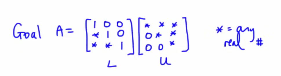
The idea behind LU factorization is to write the coefficient matrix
Once we have this factorization, we solve the system:
by first solving
which is forward substitution
and then solving :
which is backward substitution
So let's work first on understanding how to find :
with an example here.
So with this example matrix
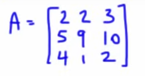
(the
or
Note that the matrix
1. Finding
So we start by finding
That can be done by simply using Gauss elimination method.
We set the pivot to
So for
So $$R_2 \ \to R_2 \ - \ \frac{5}{2} \ R_1$$
So the matrix becomes :
Now for
So $$R_3 \ = \ R_3 \ - \ 2R_1$$
So the matrix becomes:
Now for the
So :
Then :
So the matrix
2. Finding
Now the matrix
The upper triangular half of
Now the lower triangular half, which represents the
So we currently have
Now we will just fill in the gaps using the
So, for the
Next, for the
And lastly, for the
And this the
Matrix Completion
What is Matrix Completion?
Matrix completion is the process of recovering or “filling in” the missing values of a partially observed matrix.
- This is common in real data: for example, in a user-movie ratings matrix, each user has only rated a few movies, so most entries are blank.
- Matrix completion seeks to predict or estimate those unknown entries.
Why is Matrix Completion Important?
- Many large-scale data sets are incomplete (missing values), but we want to analyze or use them fully.
- It's foundational in recommender systems (Netflix, Amazon), image processing (inpainting pixels), sensor networks, social network analysis, genomics, and more.
How Does Matrix Completion Work?
-
Assume a Structure:
Usually, we assume the underlying matrix is low-rank (it can be approximated by a small number of factors or “patterns”). This is reasonable in real-world settings—user preferences, image backgrounds, etc., often vary along a few “axes.” -
Optimization Problem:
The standard matrix completion task can be stated as:Find
that minimizes subject to matching the known entries of the origin - But directly minimizing the rank is NP-hard (computationally infeasible).
-
Convex Relaxation (Nuclear Norm Minimization):
-
Instead, replace rank with nuclear norm (sum of singular values).
-
Solve:
-
This is convex and efficiently solvable; the filled matrix will have naturally low rank.
-
-
Alternating Minimization & Factorization:
- Alternatively, directly factor the matrix as
and optimize and to best fit the observed values.
- Alternatively, directly factor the matrix as
-
Algorithms:
- Singular Value Thresholding (SVT)
- Alternating Direction Method of Multipliers (ADMM)
- Gradient Descent-based methods
- (And others suited to large and/or sparse data)
Applications
- Recommender Systems: Completing the ratings matrix to recommend new items to users.
- Image & Video Processing: Restoring missing/corrupted pixels.
- Network Analysis: Recover missing links or node attributes in a graph.
- Genomics/Bioinformatics: Filling in missing gene expression values.
- Sensor Networks: Locating nodes given partial distance information.
Practical Example
Suppose
Matrix completion tries to estimate the “?” values using the assumption that MM has some low-rank structure (e.g., the ratings are mostly explained by a few genres or user types).
The Big Picture
-
Matrix completion is a generalization of matrix factorization: not only do we approximate data as
, but we also impute missing entries to create a coherent, full matrix based on observed structure. -
Modern machine learning and data science often depend on being able to recover full data matrices from incomplete samples—matrix completion is the main tool for this job.
Methods of matrix completion.
1. Gradient Descent
This method is a crucial starting point to get into the deeper echelons of machine learning.
Pre-requisites : Partial differentiation, partial differentiation chain-rule and the formula for calculating the gradient of a given function.
https://www.youtube.com/watch?v=JAf_aSIJryg&list=PLF-vWhgiaXWNi9OuPCbguaPgL67XH7crm&index=2 (Partial derivatives)
https://www.youtube.com/watch?v=XipB_uEexF0&list=PLF-vWhgiaXWNi9OuPCbguaPgL67XH7crm&index=3 (Partial derivatives chain rule)
https://www.youtube.com/watch?v=CnVes9TdnPo&list=PLF-vWhgiaXWNi9OuPCbguaPgL67XH7crm&index=9 (Gradient)
So, let me just go ahead and list the formula for the gradient of a function.
Gradient
The gradient of a scalar field
For a 2D scalar field, that would be :
A small example:
Let's say we have a scalar function:
We have to find it's gradient at points
Finding each partial derivative:
Final gradient:
What is Gradient Descent?
Gradient Descent is an iterative optimization algorithm widely used in machine learning to minimize loss (cost) functions.
The core idea:
- Start at a random point (guess for parameters/weights).
- Move in the direction of steepest descent (the negative of the gradient).
- Keep repeating until you reach the minimum or can't get lower.
It’s like walking downhill: you keep stepping in the direction that slopes most steeply down, each step being proportional to how steep the surface is beneath your feet.
Now you might be wondering, what is a loss function?
A loss function is like a "scorekeeper" for a machine learning model. It tells us how far off the model’s answers (predictions) are from the real, correct answers.
- If the model's guess is close to the true answer, the loss is small (good!).
- If the guess is very wrong, the loss is big (bad!).
During training, the model learns by trying to make this loss as small as possible. Think of it as a game where the goal is to get the lowest score!
For example, if you guessed someone’s age as 12 but they’re actually 14, your loss might be 2. If you guess 25 and they're 14, your loss is 11—much worse!
There are many types of loss functions for different tasks, but they all do the same basic job: measure how good or bad the model’s predictions are, and help the model improve by lowering that number.
The algorithm of Gradient Descent, with a step-by-step example.
Let's minimize a simple function:
- This is a parabola, shaped like a bowl, whose minimum is at
, where .
You might be wondering as to how to figure out the minimum of this function?
Simple, just put the value in
Step 1: Start with an initial guess.
Let's say
Step 2: Calculate gradient (slope)
For our function, the gradient is:
which would be:
Step 3: Iterate, update the parameter.
The update rule is:
where
Here
So a more better version of this would be:
where the original function
Step 4: Repeat till you get
Some example iterations would include
Iteration 1: x = 0.6000000000000001
Iteration 2: x = 1.08
Iteration 3: x = 1.464
Iteration 4: x = 1.7711999999999999
Iteration 5: x = 2.01696
Iteration 6: x = 2.213568
Iteration 7: x = 2.3708544
Iteration 8: x = 2.49668352
Iteration 9: x = 2.597346816
Iteration 10: x = 2.6778774528
Iteration 11: x = 2.74230196224
Iteration 12: x = 2.793841569792
Iteration 13: x = 2.8350732558336
Iteration 14: x = 2.86805860466688
Iteration 15: x = 2.894446883733504
Iteration 16: x = 2.9155575069868034
Iteration 17: x = 2.932446005589443
Iteration 18: x = 2.945956804471554
Iteration 19: x = 2.9567654435772432
Iteration 20: x = 2.9654123548617948
Iteration 21: x = 2.9723298838894356
Iteration 22: x = 2.9778639071115487
Iteration 23: x = 2.982291125689239
Iteration 24: x = 2.985832900551391
Iteration 25: x = 2.988666320441113
Iteration 26: x = 2.9909330563528904
Iteration 27: x = 2.9927464450823122
Iteration 28: x = 2.99419715606585
Iteration 29: x = 2.99535772485268
Iteration 30: x = 2.996286179882144
Iteration 31: x = 2.997028943905715
Iteration 32: x = 2.9976231551245722
Iteration 33: x = 2.9980985240996576
Iteration 34: x = 2.9984788192797263
Iteration 35: x = 2.998783055423781
Iteration 36: x = 2.999026444339025
Iteration 37: x = 2.99922115547122
Iteration 38: x = 2.9993769243769757
Iteration 39: x = 2.9995015395015807
Iteration 40: x = 2.9996012316012646
Iteration 41: x = 2.9996809852810116
Iteration 42: x = 2.999744788224809
Iteration 43: x = 2.9997958305798473
Iteration 44: x = 2.999836664463878
Iteration 45: x = 2.9998693315711025
Iteration 46: x = 2.999895465256882
Iteration 47: x = 2.9999163722055053
Iteration 48: x = 2.999933097764404
Iteration 49: x = 2.9999464782115233
Iteration 50: x = 2.9999571825692186
Iteration 51: x = 2.999965746055375
Iteration 52: x = 2.9999725968443
Iteration 53: x = 2.99997807747544
Iteration 54: x = 2.999982461980352
Iteration 55: x = 2.9999859695842814
Iteration 56: x = 2.999988775667425
Iteration 57: x = 2.99999102053394
Iteration 58: x = 2.999992816427152
Iteration 59: x = 2.9999942531417214
Iteration 60: x = 2.999995402513377
Iteration 61: x = 2.9999963220107015
Iteration 62: x = 2.999997057608561
Iteration 63: x = 2.999997646086849
Iteration 64: x = 2.999998116869479
Iteration 65: x = 2.9999984934955832
Iteration 66: x = 2.9999987947964666
Iteration 67: x = 2.999999035837173
Iteration 68: x = 2.9999992286697386
Iteration 69: x = 2.999999382935791
Iteration 70: x = 2.9999995063486327
Iteration 71: x = 2.999999605078906
Iteration 72: x = 2.9999996840631247
Iteration 73: x = 2.9999997472504996
Iteration 74: x = 2.9999997978004
Iteration 75: x = 2.9999998382403197
Iteration 76: x = 2.999999870592256
Iteration 77: x = 2.999999896473805
Iteration 78: x = 2.9999999171790437
Iteration 79: x = 2.999999933743235
Iteration 80: x = 2.999999946994588
Iteration 81: x = 2.99999995759567
Iteration 82: x = 2.999999966076536
Iteration 83: x = 2.9999999728612288
Iteration 84: x = 2.999999978288983
Iteration 85: x = 2.9999999826311865
Iteration 86: x = 2.999999986104949
Iteration 87: x = 2.9999999888839595
Iteration 88: x = 2.9999999911071678
Iteration 89: x = 2.9999999928857344
Iteration 90: x = 2.9999999943085873
Iteration 91: x = 2.9999999954468697
Iteration 92: x = 2.999999996357496
Iteration 93: x = 2.9999999970859967
Iteration 94: x = 2.999999997668797
Iteration 95: x = 2.9999999981350376
Iteration 96: x = 2.99999999850803
Iteration 97: x = 2.999999998806424
Iteration 98: x = 2.9999999990451394
Iteration 99: x = 2.9999999992361115
Iteration 100: x = 2.9999999993888893
Iteration 101: x = 2.9999999995111115
Iteration 102: x = 2.9999999996088893
Iteration 103: x = 2.9999999996871116
Iteration 104: x = 2.999999999749689
Iteration 105: x = 2.9999999997997513
Iteration 106: x = 2.999999999839801
Iteration 107: x = 2.9999999998718407
Iteration 108: x = 2.9999999998974727
Iteration 109: x = 2.999999999917978
Iteration 110: x = 2.9999999999343823
Iteration 111: x = 2.999999999947506
Iteration 112: x = 2.9999999999580047
Iteration 113: x = 2.9999999999664038
Iteration 114: x = 2.999999999973123
Iteration 115: x = 2.999999999978498
Iteration 116: x = 2.9999999999827986
Iteration 117: x = 2.999999999986239
Iteration 118: x = 2.999999999988991
Iteration 119: x = 2.999999999991193
Iteration 120: x = 2.999999999992954
Iteration 121: x = 2.999999999994363
Iteration 122: x = 2.9999999999954907
Iteration 123: x = 2.9999999999963927
Iteration 124: x = 2.9999999999971143
Iteration 125: x = 2.9999999999976916
Iteration 126: x = 2.9999999999981535
Iteration 127: x = 2.999999999998523
Iteration 128: x = 2.9999999999988183
Iteration 129: x = 2.9999999999990545
Iteration 130: x = 2.9999999999992437
Iteration 131: x = 2.999999999999395
Iteration 132: x = 2.999999999999516
Iteration 133: x = 2.9999999999996128
Iteration 134: x = 2.99999999999969
Iteration 135: x = 2.999999999999752
Iteration 136: x = 2.999999999999802
Iteration 137: x = 2.9999999999998415
Iteration 138: x = 2.999999999999873
Iteration 139: x = 2.9999999999998983
Iteration 140: x = 2.9999999999999187
Iteration 141: x = 2.999999999999935
Iteration 142: x = 2.999999999999948
Iteration 143: x = 2.9999999999999583
Iteration 144: x = 2.9999999999999667
Iteration 145: x = 2.9999999999999734
Iteration 146: x = 2.9999999999999787
Iteration 147: x = 2.999999999999983
Iteration 148: x = 2.9999999999999867
Iteration 149: x = 2.9999999999999893
Iteration 150: x = 2.9999999999999916
Iteration 151: x = 2.9999999999999933
Iteration 152: x = 2.9999999999999947
Iteration 153: x = 2.9999999999999956
Iteration 154: x = 2.9999999999999964
Iteration 155: x = 2.9999999999999973
Iteration 156: x = 2.999999999999998
Iteration 157: x = 2.9999999999999982
Iteration 158: x = 2.9999999999999987
Iteration 159: x = 2.999999999999999
Iteration 160: x = 2.999999999999999
I took the liberty to cook up a python script to see exactly in how many iterations we can get as close as possible to the minimum,
It took a total of 159 iterations to be exact. Which is why iterative methods are best left to computers, but the knowledge is still needed, hence why I added this method.
Code (for the curious cat):
pip install numpy matplotlib
import numpy as np
import matplotlib.pyplot as plt
# Function and its derivative
def f(x):
return (x - 3) ** 2
def df(x):
return 2 * (x - 3)
# Gradient descent parameters
x = 0.0 # Starting point
learning_rate = 0.1
iterations = 200 # feel free to tweak this parameter.
x_history = [x]
f_history = [f(x)]
for i in range(iterations):
grad = df(x)
x = x - learning_rate * grad
x_history.append(x)
f_history.append(f(x))
print(f"Iteration {i+1}: x = {x}")
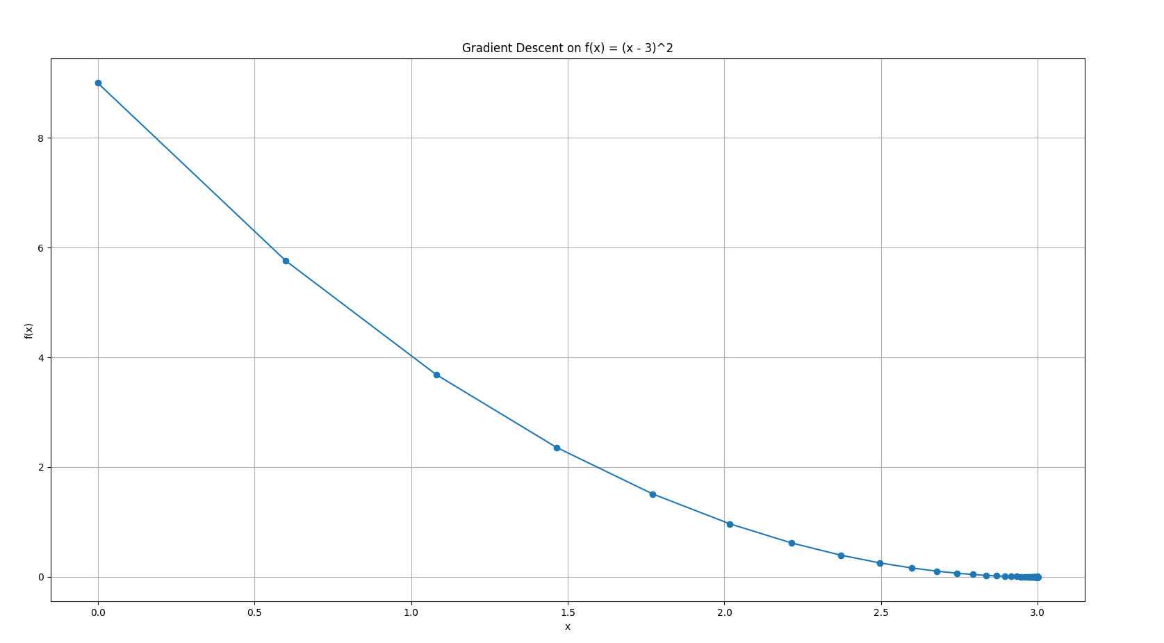
# Plotting
plt.plot(x_history, f_history, marker='o')
plt.title('Gradient Descent on f(x) = (x - 3)^2')
plt.xlabel('x')
plt.ylabel('f(x)')
plt.grid(True)
plt.show()
Step 5 : Plot the iterations.
Again, best left to computers.
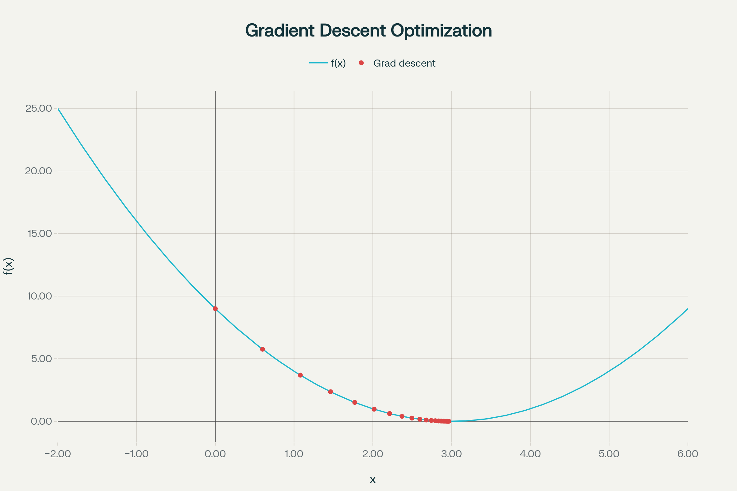
- The blue curve is
. - Red dots show each gradient descent step.
- You see how the steps start large (when farther away and the slope is steep), and get smaller as you approach the minimum.
Or a shortened one:
Types of Gradient Descent
- Batch Gradient Descent: Compute the gradient using the whole dataset before each update.
- Stochastic Gradient Descent (SGD): Update with the gradient from one example at a time.
- Mini-batch Gradient Descent: Updates with gradient from a small random subset (mini-batch); the most popular in practice.
How does Gradient-Descent tie to Matrix completion?
-
Low-Rank Factorization:
- We approximate your incomplete matrix
as , where and are low-rank factor matrices. - These are initialized randomly (or with small values).
- We approximate your incomplete matrix
-
Define the Objective (Loss) Function:
-
==The goal is to minimize the reconstruction error—the difference between the observed values in
and the corresponding entries ==in . -
Only the observed entries are included in the loss calculation.
(Don't worry about this scary lookin ahh equation. This is a given loss function, not something we need to come up with)
-
-
Gradient Descent Steps:
- At each iteration, calculate the gradient of the loss with respect to all elements of
and . - Update
and by moving a small step in the direction that most reduces the loss (as you learned for scalar functions).
- At each iteration, calculate the gradient of the loss with respect to all elements of
-
Fill in the Blanks:
- After several iterations,
and converge to values that make match the observed data well. - The missing entries (previously blanks in
) are now predicted by the corresponding entries in
- After several iterations,
Key Details
- The gradient computation only sums over observed entries, so missing elements don’t affect the update.
- The process is fully iterative: continual updates using gradients until convergence (reconstruction error stops improving).
Visualization
This chart shows how the error decreases as the algorithm proceeds—just like the basic gradient descent you experimented with, but applied to the matrix recovery problem:
Gradient Descent iterative convergence in matrix completion
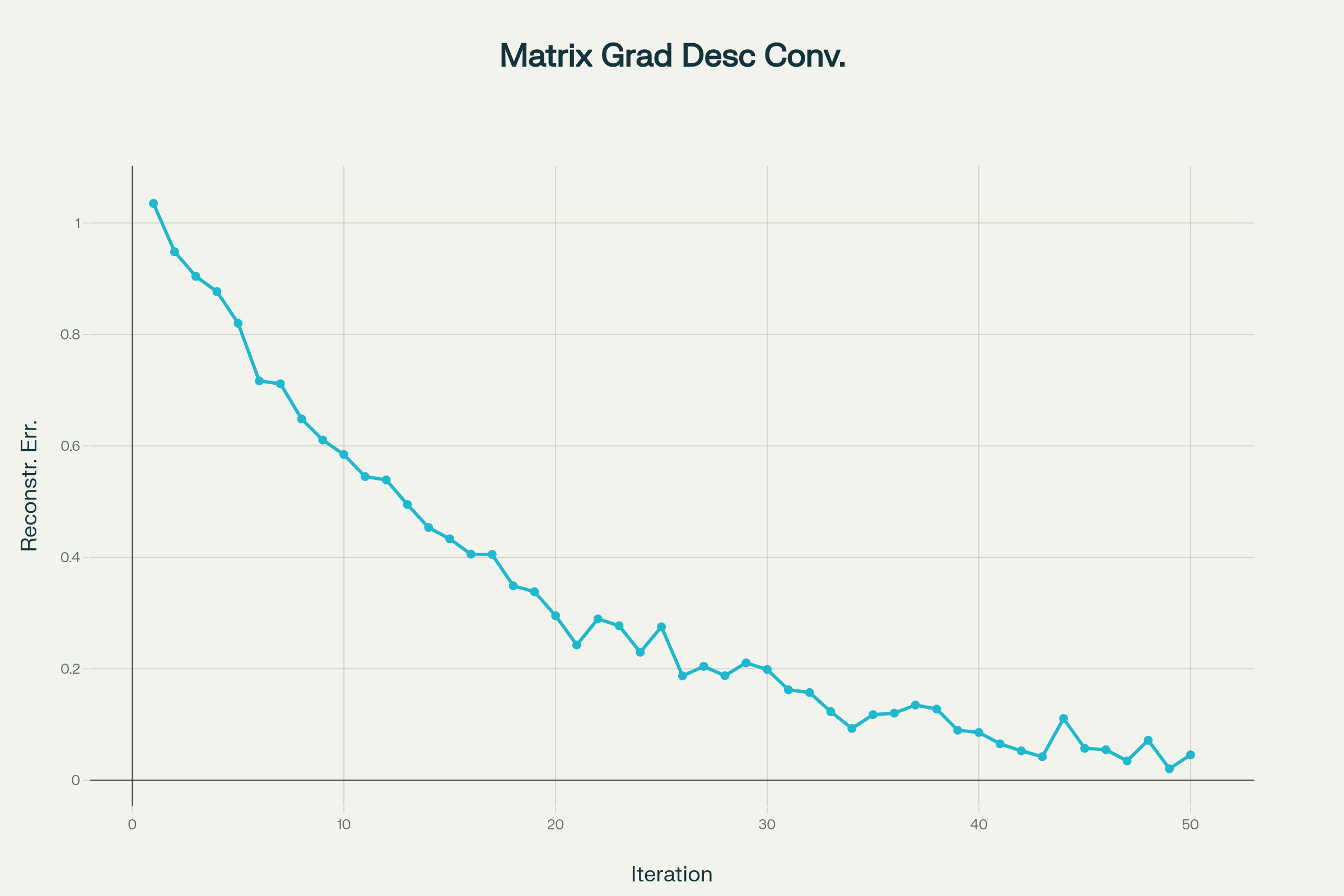
See how the error in reconstruction drops over time?
Summary
- Gradient descent enables matrix completion by optimizing the low-rank approximation only over known data points, using the same principles of gradient descent we already learned in the previous example.
- This approach allows scalable, practical recovery of missing data and is widely used in collaborative filtering and modern recommender systems.
Generative Models
Now we are slowly getting there.
For people who just want to get over this module with, here's a brief summary:
Latent Factor Models: Readable Notes (Essentials Only)
-
Latent factors are hidden variables that explain observed data. The idea: Observed features (like user ratings for movies) are influenced by a small set of hidden factors (like “action lover”, “comedy fan”).
-
Key examples:
- Matrix Factorization for recommender systems (
): Each user and item is represented by a small set of latent features. - Factor Analysis: Observed variables are modeled as linear combinations of these latent factors plus noise.
- Matrix Factorization for recommender systems (
-
Why important in ML:
- Helps find underlying structure in high-dimensional data.
- Powers recommendation engines, collaborative filtering, and dimensionality reduction.
- For your syllabus: Know that matrix factorization and factor analysis are core types; you don’t need to derive their formulas, just know they explain data with hidden, unobserved features.
Mixture Models: Readable Notes (Essentials Only)
-
Mixture model: Data comes from multiple subgroups or distributions (components), but for each point, we don’t know which group it came from.
-
Key Example:
- Gaussian Mixture Model (GMM): Each data point comes from one of several normal distributions, chosen with some probability.
-
How it works (big picture):
- Uses “soft” assignment: Each point has a probability of belonging to each group, not just one hard label.
- Fitted using the Expectation-Maximization (EM) Algorithm: Alternates between guessing assignments and updating subgroup statistics.
-
Why important in ML:
- Used for soft clustering (unlike K-means).
- Models data where groups overlap, or the origin is uncertain.
- You only need to know the concept—data is a mix of unknown sources, and EM is used to estimate the subgroups and assignments.
Bare Minimum for Exams & ML Progress
-
Know the concepts:
- Latent factor = hidden variable/feature, explains observed data.
- Mixture model = data from multiple subpopulations, with hidden labels about origin.
-
Main uses:
- Latent factor models: recommendations, finding structure, reducing dimensions.
- Mixture models: soft clustering, density estimation.
-
Very basic workflow:
- Mixture models: Use EM to alternate “guessing group” and “updating parameters.”
- Latent factor models: Find lower-dimensional structure (“features behind the data”).
Note : This is only to end the module.
A detailed section on Generative Models (Latent factor and mixture models plus a LOT more will be added in a separate pdf, outside of the syllabus, for those who want to know more in-depth)