Module 3 -- ML Model evaluation, Statistical Learning, Ensemble methods
Index
- Evaluating Machine Learning algorithms
- 3. Key Evaluation Metrics
- Introduction to Statistical Learning Theory
- The Key Ideas
- The relationship between Expected (True) risk and the Empirical Risk
- For the even more curious What is the Law of Large Numbers(LLN) and how is it related to Statistical Learning?
- Ensemble Methods
- 1. Boosting
- Boosting Algorithms AdaBoost
- 2. Bagging
- Bagging vs. Boosting Key Points
- Bagging Algorithm Random Forests
Evaluating Machine Learning algorithms
1. Why Evaluate?
To understand if your ML model:
- Actually learns useful patterns from data.
- Will generalize well to new, unseen data (not just what it was trained on).
2. The Train/Test Split
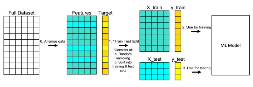
- Training set: For fitting (learning) the model.
- Testing set: For evaluating how well it works on new data.
- Sometimes, we also use a validation set to tune hyperparameters without touching the test set.
3. Key Evaluation Metrics
This content is taken from data mining module 4 from semester 6. Module 4 -- Data Streams -- Data Mining#Class Imbalance Problem
The evaluation metrics are the same since that's practically a part of ML itself.
In class imbalance, you're usually trying to detect a rare but important event, like fraud (positive class). So, accuracy becomes meaningless. We use more targeted metrics.
1. Using a Confusion Matrix
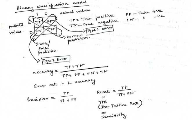
A confusion matrix is a table that displays the performance of a classification model by comparing its predictions to the actual labels of the data, especially highlighting the counts of correct and incorrect predictions for each class. This helps analyze where the model is struggling, particularly with under-represented classes, and is crucial for understanding the model's effectiveness in imbalanced datasets.
A confusion matrix summarizes predictions:
| Truth | Predicted Positive | Predicted Negative |
|---|---|---|
| Actual Positive(Spam) | TP(True Positive) (Actually predicted spam) | FN(False Negative) (False predicted as not spam) |
| Actual Negative(Not spam) | FP(False Positive) (False predicted as spam) | TN(True Negative) (Correctly predicted as not spam) |
A confusion matrix is often used in binary classification problems, where operating under class imbalance, ML models often classify differently than what's expected between two categories.
Example:
Imagine we have 100 test samples:
- 10 are actual positive (e.g., fraud)
- 90 are actual negative (e.g., normal)
Let’s assume:
-
Out of the 8 predicted as fraud:
- 5 were truly fraud → ✅ True Positives (TP) = 5
- 3 were normal but wrongly flagged → ❌ False Positives (FP) = 3
So among the 90 actual normal cases:
- 3 were misclassified → FP = 3
- So, the remaining 87 were correctly predicted as normal → ✅ True Negatives (TN) = 87
And among the 10 actual frauds:
- 5 were detected → TP = 5
- 5 were missed and wrongly predicted as normal → ❌ False Negatives (FN) = 5
So this is our confusion matrix:
| Truth | Predicted Positive | Predicted Negative |
|---|---|---|
| Actual Positive | TP = 5 | FN = 5 |
| Actual Negative | FP = 3 | TN = 87 |
2. Precision (a.k.a Positive Predictive Value)
Precision answers the important question of:
"Out of all the cases I predicted as positive, how many were actually positive?"
- High precision means: When the model says "fraud," it’s usually right.
- Important when false positives are costly (e.g., spam filters, arresting people).
I mean, you wouldn't someone to be wrongly arrested, or your mail system to wrongly classify an important email as spam, right?.
3. Recall (a.k.a Sensitivity / True Positive Rate)
Recall answers this important question:
"Out of all the actual positives, how many did I catch?"
- High recall means: The model catches most of the actual frauds.
- Important when missing positives is dangerous (e.g., fraud detection, cancer screening).
You most certainly wouldn't want to miss a fraud detection, or a cancer screening, right?
4. F1 Score (harmonic mean of precision and recall)
"Balance between precision and recall"
- F1 score is useful when you want balance and care about both FP and FN.
- It punishes extreme imbalance (e.g., very high precision but very low recall).
So in our case, from the confusion matrix, we see that:
| Truth | Predicted Positive | Predicted Negative |
|---|---|---|
| Actual Positive | TP = 5 | FN = 5 |
| Actual Negative | FP = 3 | TN = 87 |
The model detected 5 frauds (TP = 5), but:
- It missed 5 other actual frauds → FN = 5
- It also wrongly flagged 3 normal transactions as frauds → FP = 3
Then:
So what do these metrics mean?
✅ Precision = 62.5%
"Out of all the cases the model predicted as fraud, 62.5% were actually fraud."
- So 37.5% of the flagged frauds were false alarms (false positives).
- This tells us the model is moderately precise, but still wastes some effort on false positives.
📉 Recall = 50%
"Out of all the actual frauds in the data, the model only caught half of them."
- So it missed 50% of actual frauds → that's 5 real frauds left undetected.
- This is critical in domains like fraud detection or medical diagnostics, where missing positives is risky.
⚖️ F1 Score = 55.5%
"The overall balance between catching frauds and avoiding false alarms is just slightly above average."
- F1 score is not great here, because recall is dragging it down.
- It shows your model is not confident or consistent in handling fraud detection.
🔍 Summary Table
| Metric | What it measures | High when... |
|---|---|---|
| Precision | Correctness of positive predictions | FP is low |
| Recall | Coverage of actual positives | FN is low |
| F1 Score | Balance of precision and recall | Both FP and FN are low |
| Metric | Value | Interpretation |
|---|---|---|
| Precision | 62.5% | Somewhat accurate when it does say “fraud,” but makes mistakes 37.5% of the time |
| Recall | 50% | Misses half of actual fraud cases, which is risky |
| F1 Score | 55.5% | Model needs tuning — it’s mediocre at both catching frauds and being accurate |
ROC Curve & AUC
Shows trade-off between true positive rate and false positive rate at various thresholds; AUC (Area Under Curve) summarizes.
For Regression:
- Mean Squared Error (MSE):
- Mean Absolute Error (MAE):
- R² Score (Coefficient of Determination):
Fraction of variance explained by the model.
4. Cross-Validation
- K-Fold Cross-Validation:
- Split data into K parts (“folds”)
- Train on K-1 folds, test on the remaining fold
- Repeat K times, with each fold used as test set once; average results.
- Why?
- Helps ensure results aren’t due to a “lucky” or “unlucky” train/test split.
- Gives a more robust, general performance estimate.
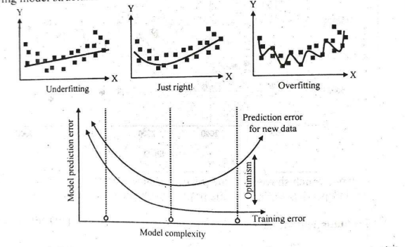
5. Overfitting & Underfitting
-
Overfitting: Model learns noise in training data; performs poorly on new data.
-
Underfitting: Model is too simple to capture signal; poor performance on both train and test data.
-
Diagnostic: High training accuracy + low test accuracy = overfitting. Low accuracy on both = underfitting.
6. Key Strategies for Fair Evaluation
- Always evaluate on unseen data.
- Use cross-validation for limited data.
- Compare models using the same data splits.
- Be mindful of imbalanced data: accuracy alone can be misleading; emphasize precision, recall, or F1 for unbalanced classes.
Example.
Let's understand this better with the help of an example.
Let's say we have a dataset of house prices:
| Size (sqft) | Price (₹) |
|---|---|
| 1000 | 70,000 |
| 1200 | 80,000 |
| 1300 | 85,000 |
| 1500 | 95,000 |
| 1800 | 115,000 |
Let’s split this into train and test:
-
Train Set (80%):
- (1000, 70,000), (1200, 80,000), (1300, 85,000), (1500, 95,000)
-
Test Set (20%):
- (1800, 115,000)
Fitting a regression model (let's say, linear regression)
Assume we use a simple linear regression model:
-
We fit this model to the train set data (training over a bunch of epochs)
-
Suppose after fitting, we get:
-
-
-
So, the regression equation is:
-
Make predictions on the test set.
- For Size of
:
Calculate Evaluation Metrics
a) Mean Squared Error (MSE)
MSE is the average of the squared differences between actual values and predicted values. It is a common metric for measuring the accuracy of regression models in statistics and machine learning—a lower MSE means better model predictions.
Here's what each symbol means:
: Number of observations (data points) in your dataset. : The actual or true value of the -th data point. : The predicted value from your model for the -th data point. (summation symbol): Indicates that you sum across all data points from 1 to . : The error or residual for each observation (difference between actual and predicted). - (yᵢ - ŷᵢ)²: Square of the error for each observation.
For our test point:
b) Mean Absolute Error (MAE)
c) Coefficient of Determination (
where
- For one test point,
is not meaningful, but with more data, it tells what fraction of the variance in our model explains (ranges from -∞ to 1, with 1 being perfect prediction).
Summary Table
| Metric | Formula | Example Value |
|---|---|---|
| MSE | 25,000,000 | |
| MAE | ||
| R² Score | Not meaningful here |
Key Takeaways
- Step 1: Split data → train/test.
- Step 2: Fit regression model to train set.
- Step 3: Predict test set values.
- Step 4: Calculate MSE, MAE, R² to measure performance (lower MSE/MAE, higher R² = better!).
Introduction to Statistical Learning Theory
Essential Prerequisites (for those who want to dive even deep)
-
Basic Probability & Statistics
- Random variables, probability distributions (especially joint and conditional)
- Expectation, variance, and basic properties of estimators
-
Calculus and Linear Algebra
- Differentiation, integration (especially for defining and minimizing risk/loss)
- Vector and matrix arithmetic (for handling high-dimensional data, but not deep theory at first)
-
Core Machine Learning Workflow Concepts
- Training set vs. test set (i.i.d. sampling from a distribution)
- Hypothesis space: the set of candidate functions/models under consideration
- Loss/risk function: how we measure the “cost” of a particular prediction or model
What is Statistical Learning Theory?
Statistical Learning Theory is the theoretical backbone of modern machine learning. It studies and explains:
- How algorithms can learn patterns from data,
- How to predict or generalize well to new data (not just the training set)
- How to balance model complexity and accuracy to avoid both underfitting and overfitting.
The Key Ideas
1. Learning from Data Means Function Approximation
-
You get a set of input-output pairs (
), drawn from some unknown joint probability distribution -
You want to find a function
(your model) that predicts as accurately as possible. For simplicity purposes, we will assume that the model is a linear regression one.
2. Risk (Error) and Loss Functions
Loss Function
We already know about the Loss Function from the Module 2 -- Unsupervised Learning -- Machine Learning#What is Gradient Descent? section.
Still I will re-iterate here again.
A loss function is like a "scorekeeper" for a machine learning model. It tells us how far off the model’s answers (predictions) are from the real, correct answers.
- If the model's guess is close to the true answer, the loss is small (good!).
- If the guess is very wrong, the loss is big (bad!).
During training, the model learns by trying to make this loss as small as possible. Think of it as a game where the goal is to get the lowest score!
We denote this loss function by
- Example : Squared loss (
) or classification error, can be ( , if correct, and there is virtually no loss, or if wrong, and the loss is very high.). The loss value is clamped between and .
Risk Functions
Expected Risk (true risk):
It's defined a multi-variable integral of the product of the loss function and some unknown joint probability distribution.
- The true average loss over all possible data is usually unknown, since
is usually unknown.
Empirical Risk :
- The average loss on the training set. Now this, we can compute.
3. Empirical Risk Minimization (ERM)
-
In practice, we choose
from a set of possible models ( , or “hypothesis space”) to minimize empirical risk—because we only have a finite sample. - This is the logic behind nearly all ML algorithms (least squares regression, SVMs, neural nets, etc.).
4. Generalization: Why Not Just Memorize the Training Data?
- A model that just remembers the training set isn’t useful; it must work well on new data.
- Overfitting: When a model fits the training data too closely and performs poorly on new data.
- Underfitting: When a model is too simple to capture the patterns, so it performs poorly everywhere.
5. Bias-Variance Tradeoff
- Simpler models have high bias (might miss patterns—underfit).
- Complex models have high variance (fit noise—overfit).
- Goal: Find a “sweet spot” (right complexity), where performance on new data is best.
6. Capacity and Hypothesis Space
- The set of models you consider (
) defines the complexity/capacity of learning: - Larger
: More expressive, but higher risk of overfitting. - Smaller
: Less expressive, but safer from overfitting.
- Larger
Example
Let's dive deeper into this and fully explore the terminologies as well as how to calculate the empirical risk with an example.
Main difference between Expected (True) Risk and Empirical Risk
We already know from Risk Functions :
Expected Risk (true risk):
It's defined a multi-variable integral of the product of the loss function and some unknown joint probability distribution.
- The true average loss over all possible data is usually unknown, since
is usually unknown.
Empirical Risk :
- The average loss on the training set. Now this, we can compute.
The relationship between Expected (True) risk and the Empirical Risk
-
The empirical risk is an approximation of the expected risk. As you get more data, and if your data is independent and identically distributed (i.i.d.), empirical risk converges to the expected risk (Law of Large Numbers).
-
But: Empirical risk is always based on a sample, so it can be too optimistic if the model overfits ("memorizes") the training data. That's why generalization is critical.
Calculating and Minimizing the Empirical Risk
Suppose a Regression problem:
- Data
or
| 1 | 2 |
| 2 | 4 |
| 3 | 6 |
- Hypothesis(
) or the model chosen : A simple linear model
where
Step 1: Calculate Empirical Risk
The empirical risk is calculated using the formula:
Where the loss function,
Now a small detour:
Why this specific loss function?
Generally for exams and standard ML projects, the loss function is chosen primarily based on the type of machine learning problem, not on the specific model (hypothesis) itself. There are “de-facto” (case specific) default losses for most tasks:
General Loss Function Selection Rules
1. Regression Problems
-
Default loss: Mean Squared Error (MSE)
- Measures the average squared difference between predicted and actual values.
-
Alternatives:
- Mean Absolute Error (MAE): Less sensitive to outliers.
- Huber loss: Compromise, robust to outliers but differentiable for optimization.
2. Classification Problems
-
For binary classification:
- Default: Binary Cross-Entropy (also called Log Loss)
-
For multiclass classification:
- Default: Categorical Cross-Entropy
3. Other Specialized Losses
- For class imbalance: Weighted cross-entropy, focal loss, etc.
- For metric learning, segmentation, etc.: Triplet loss, Dice loss, etc..arxivarxiv
Exam and Coursework Perspective
-
For typical exam questions:
-
If not specified, use Mean Squared Error for regression, and Cross-Entropy for classification.
-
You do not need to justify changing the loss function unless the question mentions special needs (like outliers or custom objectives).
-
Always mention the loss you’re using and why: “For regression tasks, we minimize the standard mean squared error loss, since it penalizes large errors and is the most widely used default loss for continuous targets.”
-
In Summary
-
Default loss functions are usually the right choice for exams and general practice.
-
The choice is based on the type of problem (regression/classification) and (rarely, for advanced courses) on the data's unique properties.
-
For introductory and university-level exams, expect to use:
- MSE or MAE for regression
- Cross-Entropy for classification
No need to deeply justify or derive the loss unless asked specifically; simply state the common standard and proceed with your calculations or explanations.
Now, coming back to the example:
And
So, the empirical risk becomes:
Now, we expand:
Now this is our current empirical risk.
Step 2: Now, we minimize the empirical risk (Empirical Risk Minimization (ERM)).
The goal of empirical risk minimization (ERM) is to find a model that minimizes this sample-based risk, hoping it also performs well on unseen data.
We need to find a new weight
This is the same as solving the linear least squares regression method from
Module 3 -- Time Series Mining#a. Linear Trend (Recap)#How to calculate
whose proper formula for this purpose is:
So:
What does this mean?
This means that the empirical risk minimizer is
Why?
-
In reality, if we had infinite data covering every possibility, minimizing expected risk would be ideal.
-
With finite data, we "stand in" for true risk by minimizing the empirical risk computed on the dataset we have.
For the even more curious: What is the Law of Large Numbers(LLN) and how is it related to Statistical Learning?
https://www.geeksforgeeks.org/maths/law-of-large-numbers/
This will help you understand how Empirical Risk Minimization (ERM) is based on LLN and how it gets very close (converges) as the number of trials and observations (or experiments) (epochs in training) increases.
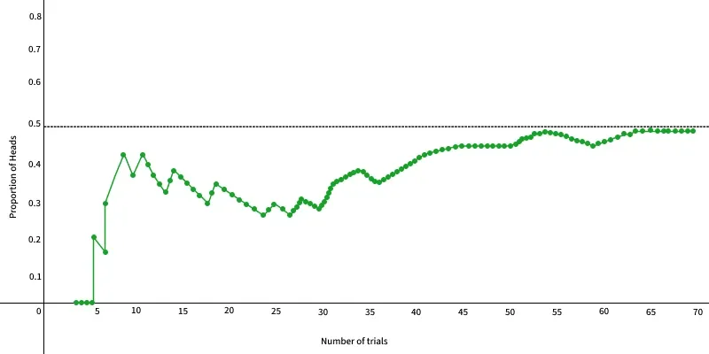
The Law of Large Numbers (LLN) is a mathematical theorem in probability and statistics that helps us understand how averages work over time. It states that if an experiment is repeated many times, the average result will approach the expected value more closely.
Law of Large Numbers states that the average is closer to the expected or theoretical value as the number of trials or observations increases.
**For example: if you flip a fair coin many times, the proportion of heads and tails will get closer to 50% each.
In the graph below, we can see how the proportion of heads approaches 0.5 as the number of trials increases.
Example explaining the law of large numbers: Imagine your bag contains blue and red balls- 50% red, 50% blue.
-
If you draw just one ball, it could be red or blue — there's no way to predict the exact outcome, and that single draw doesn’t tell you much about the overall mix in the bag.
-
Now suppose you draw 10 balls one by one, noting the color each time. You might get 6 red and 4 blue, or maybe 7 red and 3 blue. The ratio likely won’t be exactly 50:50, but it’ll be close.
-
Now imagine repeating this process hundreds or even thousands of times. As your sample size grows, the proportion of red to blue balls in your recorded results will get closer and closer to the actual 50:50 ratio in the bag.
So, in summary:
The more trials you perform, the closer your observed average (or proportion) gets to the true theoretical value.
Now, while minimizing the empirical risk in statistical learning, the goal of empirical risk minimization (ERM) is to find a model that minimizes this sample-based risk, hoping it also performs well on unseen data.
Convergence of empirical risk towards real risk due to LLN
The convergence of empirical risk to actual risk stems directly from LLN. As the number of training samples increases, the empirical risk
Limitations of the Law of Large Numbers
If you are not interested in this section then you can skip ahead to Ensemble Methods
Various limitations of the Law of Large Numbers are:
-
Sample Size: When the sample size is genuinely huge, the Law of huge Numbers operates most effectively. A limited sample size could mean that the results do not represent the underlying population and that the law does not hold.
-
Independence: The Law of Large Numbers presupposes that the events or observations are unrelated to one another. The law might not apply correctly if there is any dependence or correlation between the observations.
-
Rate of Convergence: The Law of Large Numbers states that as the sample size grows, the sample mean will converge to the population mean, but it doesn't say how quickly this convergence will happen. Sometimes, the convergence could be sluggish, and a huge sample size might be needed to get the appropriate degree of precision.
-
Outliers and Extreme Values: The existence of outliers or extreme values in the data can have a significant impact on the Law of Large Numbers. Even with a high sample size, a few extreme observations can considerably affect the sample mean.
-
Observations Not Identically Distributed: The Law of Large Numbers presupposes that the data come from a single probability distribution. The law might not hold if the underlying distribution varies over time or if the data are drawn from disparate distributions.
-
Biased Sampling: Law of Large Numbers may not apply, and the sample mean may not converge to the true population mean if the sampling procedure is biased or non-random.
-
Finite Population:* In general, an infinite population is used to state the Law of Large Numbers. The law might need to be changed or altered when working with a finite population to take into consideration the population's finite size.
Applications of LLN in Computer Science
The Law of Large Numbers (LLN) is widely used in Computer Science, especially in areas involving randomness, estimation, and simulation. Some of the key applications are:
-
Monte Carlo Simulations: A technique that uses repeated random sampling to estimate numerical results used in graphics rendering, AI game engines, risk analysis, and optimization problems (which itself is based on Markov Chains, another beast in Probability and Statistics.)
-
Probabilistic Algorithms: Algorithms like Randomized QuickSort, Las Vegas use randomness.
-
Distributed Systems: Random sampling is used for decisions like which server to assign a task to.
-
Load Balancing: LLN helps predict that, over time, the load will distribute evenly, assuming fair randomness.
-
Machine Learning: LLN supports the reliability of training data with more data, and sample statistics (like mean or variance) converge to true population values.
-
Network Traffic Analysis: Used to estimate average latency, packet loss, or throughput over time.
Ensemble Methods
What are Ensemble Methods?
Ensemble methods in machine learning are techniques that combine multiple individual models, known as base learners, to create a single, more accurate and robust predictive model.
The fundamental principle here is that a group of models working together can outperform any single model, leveraging the strengths and mitigating the weaknesses of individual models.
Methods of Ensemble Learning
1. Boosting
Boosting is an ensemble learning technique that combines multiple weak learners (often simple models like shallow decision trees) into a single strong learner that achieves higher accuracy and reduced bias than any individual weak model.
How Does Boosting Work?
-
Sequential Learning:
Boosting trains a series of weak learners one after another, each focusing on the errors (or difficult examples) made by the last. -
Weighted Emphasis:
Each new model pays more attention (increases the weights) to the training samples that were previously misclassified or predicted with large error. Source: gfg-adaboost -
Aggregation:
The outputs of all weak learners are combined (typically through a weighted sum or majority vote) to form the final model prediction.
General Steps in Boosting
-
Initialize Weights:
All training samples start with equal weights. -
First Weak Learner:
Train a simple model (e.g., decision stump) on the data using these weights. -
Update Weights:
Increase weights for samples misclassified by this model, decrease for correctly classified ones. -
Next Weak Learner:
Train a new model that focuses more on the updated (harder) samples. -
Repeat:
Continue steps 3–4 for a fixed number of rounds or until performance plateaus. -
Combine:
Aggregate the weak models’ outputs (using learned weights) to give the final prediction.
Why Use Boosting?
-
Reduces Bias:
Transforms underfitting simple models into a strong model by learning from mistakes. -
Works Well for Many Problems:
Used in classification, regression, ranking, etc. -
Adaptive:
Automatically focuses on “hard” cases where earlier models failed.
Key Types of Boosting Algorithms
-
AdaBoost (Adaptive Boosting):
The classic form; increases weights on misclassified points and combines weak classifiers with confidence-weighted votes. -
Gradient Boosting:
Each new learner fits to the residual errors of the combined previous models, optimizing a loss function using gradient descent. -
XGBoost, LightGBM, CatBoost:
Modern, scalable versions for large datasets.
Boosting Algorithms : AdaBoost
What is AdaBoost?
-
AdaBoost is a boosting algorithm that combines multiple weak learners (usually shallow decision trees called “decision stumps”) to form a single strong predictive model.
-
The power of AdaBoost is in focusing each new weak learner on the mistakes (misclassified points) of the previous ones by increasing their weight in subsequent rounds.
How AdaBoost Works (Step-by-Step)
-
Initialize Sample Weights:
- Start with all training data points weighted equally.
-
Train Weak Learner:
- Fit a simple classifier (stump) to the data using current weights.
-
Calculate Error:
- Measure the error rate (weighted sum of misclassified points).
-
Calculate Learner Weight:
-
Assign a weight (
) to the model based on how accurate it was; higher for better models. -
-
-
Update Data Weights:
- Increase weights for misclassified data.
- Decrease weights for correctly classified data.
- This forces the next weak learner to focus on the “hard” cases.
-
Repeat Steps 2–5:
- Keep adding weak learners, each time updating weights to emphasize previous errors.
-
Final Prediction (Ensemble):
- Combine weak learners’ outputs with their weights
. - Final class is usually a weighted majority vote of all learners.
- Combine weak learners’ outputs with their weights
Key AdaBoost Equations
- Error rate for weak learner
:
- Alpha(importance of the weak learner recalculation based on error rate):
- Weight Update Rule:
- where
is the new updated weight, : Positive for misclassification (needs a stronger weight), Negative for correct (keep weight as is).
Example Explanation
| Instance | Feature | True Label |
|---|---|---|
| A | 1 | +1 |
| B | 2 | +1 |
| C | 3 | -1 |
| D | 4 | -1 |
Step 1: Initialize weights
- All weights are equal; for 4 samples,
Step 2: Train first weak learner
-
Suppose the first decision stump predicts all as +1, so it misclassifies points(or instances) C and D.
-
Error rate :
- Compute
(the importance of the weak learner):
(In practice, the example would use a slightly better learner, but this illustrates the update.)
- Update the weights for C and D using the weight update rule:
So the weights stay the same.
What Does This Mean?
-
The weak learner in this case is no better than random, so it doesn’t get to influence the ensemble (total final output) (
). -
The data weights don’t change, so the next learner sees the same data emphasis.
In a Real AdaBoost Sequence
-
Usually, the weak learner does better than random. This gives
, so and weights on misclassified samples will increase. -
If a learner is much worse than random (error > 0.5), AdaBoost can flip its predictions and treat it as stronger than random.
-
In practical AdaBoost, the “stump” should always be a little better than random on the current weighted data, otherwise it adds nothing.
AdaBoost: Usages
- Classification: Excellent with tabular (structured) data and moderate noise.
- Image processing: Face detection and recognition (early successes).
- Ensemble stacking: Used as a base or meta-learner in many ML workflows.
- Robust to overfitting: When weak learners are very simple (e.g., decision stumps), AdaBoost resists overfitting.
AdaBoost: Limitations
-
Sensitive to Noisy Data:
-
Computationally Intensive:
- Many rounds of training (especially with complex learners or large datasets) can be time-consuming.
-
Not for all base learners:
- Usually works best with simple, fast weak learners; fails if base learner is too complex or inflexible.
-
Overfitting possible:
- If over-boosted (run too many rounds), or with very complex base learners, AdaBoost can overfit training data.
2. Bagging
What is Bagging?
-
Bagging (Bootstrap Aggregating) is an ensemble method that builds multiple models independently on different random subsets of the data (created via bootstrap sampling), then aggregates their results for a more robust and stable prediction.
-
Main purpose: Reduces model variance and overfitting (especially helpful for high-variance models like decision trees).
How Does Bagging Work?
-
Bootstrap Sampling:
Randomly sample the training set with replacement to create multiple different “bootstrap samples.” -
Base Learner Training (in Parallel):
Train a base learner (usually a decision tree) on each bootstrap sample—these models are independent and can be trained in parallel. -
Prediction Aggregation:
-
For classification: Use majority voting (the class predicted by most models is the final prediction).
-
For regression: Use averaging (the average prediction of all models is the final output).
-
-
Result:
The ensemble prediction is more robust (less sensitive to training data noise) than any single model.
Advantages of Bagging
- Reduces variance: Helps “unstable” base learners like decision trees generalize better—and reduces overfitting.
- Robustness: Less sensitive to data outliers/noise.
- Parallelization: Base models can be trained independently, making bagging fast with sufficient computing power.
Disadvantages of Bagging
- Does not reduce bias: If base learners are already too simple (high bias), averaging them won’t fix underfitting.
- More computation: Training multiple models requires more memory and CPU.
- Less interpretability: The ensemble (e.g., a forest of trees) is harder to interpret than a single model.
Bagging vs. Boosting: Key Points
| Aspect | Bagging | Boosting |
|---|---|---|
| Training | Parallel, independent | Sequential, dependent |
| Data Sampling | Bootstrap sampling | Reweights samples |
| Model Focus | Reduces variance | Reduces bias & variance |
| Typical Use | Random Forest | AdaBoost, XGBoost |
| Output Aggregation | Equal vote (avg) | Weighted vote |
Typical Uses
-
Random Forests: The most famous bagging-based model—applies bagging to decision trees.
-
General bagging classifiers/regressors: For any base learner (though best for those prone to overfitting).
Bagging Algorithm: Random Forests
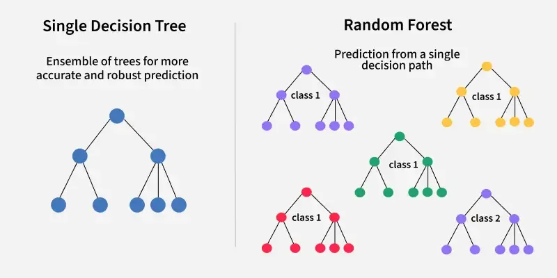
What is Random Forest?
https://www.ibm.com/think/topics/random-forest
https://www.geeksforgeeks.org/machine-learning/random-forest-algorithm-in-machine-learning/
-
Random Forest is an ensemble machine learning algorithm that builds a “forest” of many decision trees, each trained on slightly different random data and features.
-
Prediction:
-
For classification: output is the majority vote of the trees.
-
For regression: output is the average of the trees’ predictions.
-
-
Used for both classification and regression tasks.
How Does Random Forest Work?
-
Bootstrap Sampling (Bagging step):
- For each tree, generate a bootstrap sample by randomly sampling the training data with replacement.
-
Tree Building:
- Each tree is trained on its sample.
- When splitting a node, the tree considers only a random subset of features (this is the key “random” step that makes forests better than just bagging).
-
Prediction:
- For a new sample, each tree predicts.
- Classification: Final prediction is the class with most votes.
- Regression: Final prediction is the mean of all tree predictions.
-
Out-of-Bag (OOB) Error:
- Each tree leaves out about 1/3 of the data (“out-of-bag” data), used for internal validation without a test set.
Step-by-Step Example (Classification):
Suppose you have a dataset with 100 points.
-
Step 1: Generate (say) 100 bootstrap samples, one for each tree.
-
Step 2: Train 100 decision trees. Each tree:
- Uses a random subset of features at each split.
-
Step 3: For a new data point, all 100 trees predict.
- Trees vote: 55 say “A,” 45 say “B.” Final prediction: “A” (majority vote).
-
OOB Error: For each point, average the predictions from trees that did NOT see this point while training—gives a quick estimate of generalization error.
Advantages of Random Forest
- High accuracy: Combines many weak, diverse models for strong overall performance.
- Robust to overfitting: Trees are decorrelated via feature randomness and bagging.
- Handles both numeric & categorical features.
- Feature importance: Can estimate which features are most important for prediction.
- Tolerant to missing data and outliers.
- Good for very large datasets and high-dimensional problems.
Limitations of Random Forest
- Slower Inference: Predicting can be slow with many trees (compared to a single tree).
- Large in Memory: Needs to store many trees.
- Less interpretable: The decision process is a “black box” compared to a single tree.
- Does not extrapolate (in regression): Struggles with values outside the training data range.
Random Forest vs. Bagging vs. Boosting
| Aspect | Random Forest | Bagging | Boosting |
|---|---|---|---|
| Base Learner | Decision trees (with feature randomness) | Any (usually trees) | Any (usually stumps) |
| Aggregation | Majority vote/average | Majority vote/average | Weighted vote/average |
| Tree Diversity | Yes (features + data) | Some (data only) | Learners focus on errors |
| Overfitting | Lower | Lower | Risk (if overdone) |