Module 5 -- Types of Machine Learning Methods
Index
- Scalable Machine Learning (Online and Distributed Learning)
- 1. Online Learning
- 2. Distributed Learning
- 3. Semi-Supervised Learning (SSL)
- 4. Active Learning
- 5. Reinforcement Learning (RL)
- 6. Bayesian Learning
Scalable Machine Learning (Online and Distributed Learning)
1. Online Learning
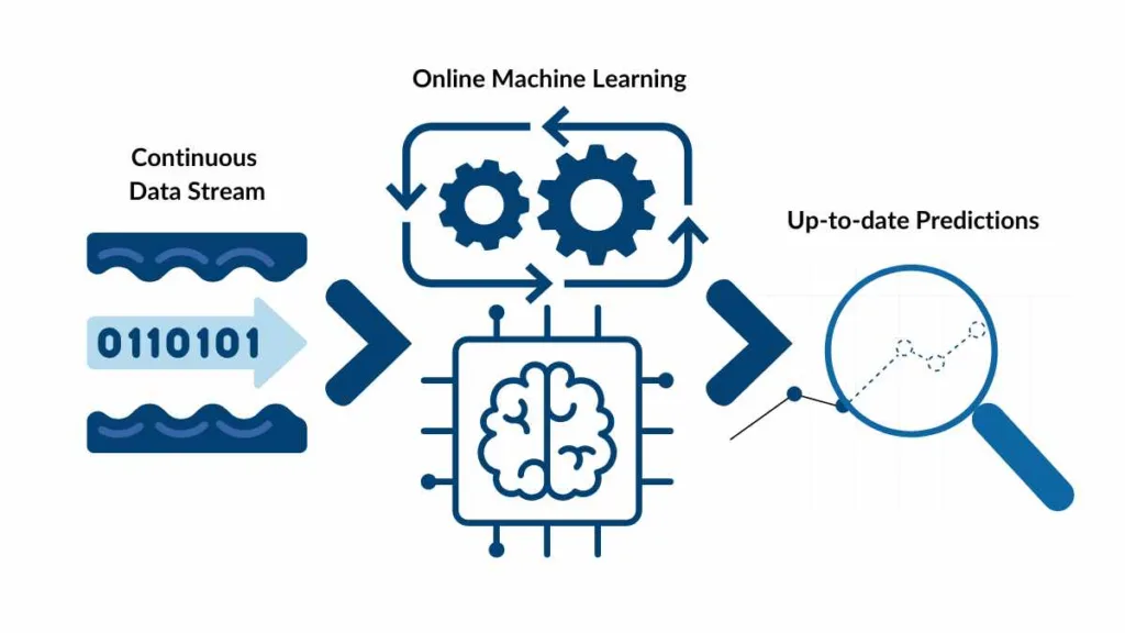
Online learning is a learning paradigm where the model updates itself incrementally, processing one example at a time, instead of training on the full dataset at once.
It is a technique where models are trained sequentially with data that arrives over time, allowing them to update continuously and adapt to new information in real-time. This contrasts with batch learning, which trains on the entire dataset at once and is useful for applications that require dynamic adaptation to evolving data, such as real-time fraud detection or e-commerce recommendations.
1.1 Why Online Learning Exists
Modern systems generate high-velocity data streams such as:
- user click logs
- sensor or IoT readings
- social media streams
- financial tick data
- continuous server logs
Storing all incoming data is often impractical.
Online learning solves this by performing training and prediction simultaneously as new examples arrive.
1.2 Core Idea of Online Learning
At each time step
- Receive input
- Predict
- Observe true label
- Update the model parameters using the loss on this single example
General weight update rule:
This is essentially stochastic gradient descent with batch size 1, allowing continuous learning.
1.3 Online vs Batch Learning
| Feature | Online Learning | Batch Learning |
|---|---|---|
| Data | Streaming / infinite | Entire dataset available |
| Updates | Every example | Full epochs |
| Memory use | Very low | High |
| Adaptation | High (handles drift) | Low |
| Update noise | High | Low |
| Convergence | Harder | Easier |
1.4 Concept Drift
Concept drift refers to changes in the underlying data distribution over time.
Examples:
- user preferences changing
- market trends shifting
- sensor wear causing different readings
- changing patterns in spam messages
Online learning adapts to drift because it updates continuously.
1.5 Types of Online Learning Algorithms
A. Perceptron Algorithm
For binary classification:
- If prediction correct → no update
- If incorrect → update using:
Uses a “mistake-driven” approach.
B. Online Gradient Descent (OGD)
General update:
Works for regression, classification, and most differentiable models.
C. Winnow Algorithm
- Uses multiplicative weight updates
- Effective when many features are irrelevant
- Popular in text-related tasks
D. Passive-Aggressive Algorithms (PA)
These algorithms update only when necessary.
- Passive: If prediction is correct with sufficient margin → no update
- Aggressive: Otherwise update just enough to correct the mistake
Used in online SVM-like methods and streaming classification.
1.6 Online Learning in Deep Learning
Streaming SGD / Mini-batch SGD
Although not “pure” online learning, deep networks often use stochastic or small-batch updates, enabling scalable training on large datasets.
Reinforcement Learning (RL)
RL agents learn online by interacting with an environment; updates are made after each step using experience samples.
1.7 Regret in Online Learning
Regret measures how much worse the online algorithm performs compared to the best fixed model in hindsight.
Good algorithms achieve sub-linear regret such as
This means they become competitive over time.
1.8 Advantages of Online Learning
- Very memory efficient
- Works with infinite streams
- Fast to update
- Handles concept drift
- Computationally cheap
- Suitable for large-scale, real-time applications
1.9 Limitations of Online Learning
- Updates are noisy
- Learning rate must be carefully tuned
- Poor initial performance until enough data seen
- Harder to parallelize
- Convergence guarantees weaker
- Can “forget” older patterns
1.10 Real-World Applications
- Real-time fraud detection
- Spam filtering systems
- Adaptive traffic control
- Realtime bidding in advertising
- Online recommendations
- Handwriting/keyboard prediction
- IoT sensor analytics
- High-frequency trading systems
1.11 Online-to-Batch Conversion (Optional but useful)
Online algorithms can be converted to batch models by:
- averaging parameters over time, or
- selecting the best hypothesis seen so far
This demonstrates theoretical power of online learning in batch settings.
2. Distributed Learning
Distributed learning refers to machine learning techniques where data, computation, or model components are spread across multiple machines (nodes) to enable faster training and to handle very large datasets or models.
It is essential when a single machine cannot store the entire dataset or cannot compute gradients fast enough.
2.1 Why Distributed Learning?
Modern ML workloads involve:
- Massive datasets (terabytes–petabytes)
- Very large models (deep networks with billions of parameters)
- Real-time applications requiring fast retraining
- Hardware limits on computation, memory, and bandwidth
Distributed learning enables scalability through parallelism and coordination across machines.
2.2 Types of Parallelism
Distributed ML typically uses two major forms of parallelism:
2.2.1 Data Parallelism
Each worker machine:
- Receives a different subset of data
- Maintains a local copy of the model
- Computes gradients on its local data
- Sends gradients to a central coordinator
- Parameters are updated and synchronized across all workers
This approach is effective when:
- The model fits in memory of a single machine
- The dataset is too large or training is too slow on one system
Gradient Update Concept
If worker
Then updates parameters:
This allows multiple machines to train the same model simultaneously.
2.2.2 Model Parallelism
Used when the model itself is too large to fit on a single machine.
Two main ways to split a model:
- Layer-wise partitioning:
- Machine 1 holds layer 1
- Machine 2 holds layer 2
- and so on
- Tensor / weight partitioning:
- Large weight matrices split across machines
Each machine computes part of the forward and backward pass.
Useful for:
- Very large transformer models
- Huge embedding tables
- Large-scale deep learning architectures
2.3 Key Distributed Architectures
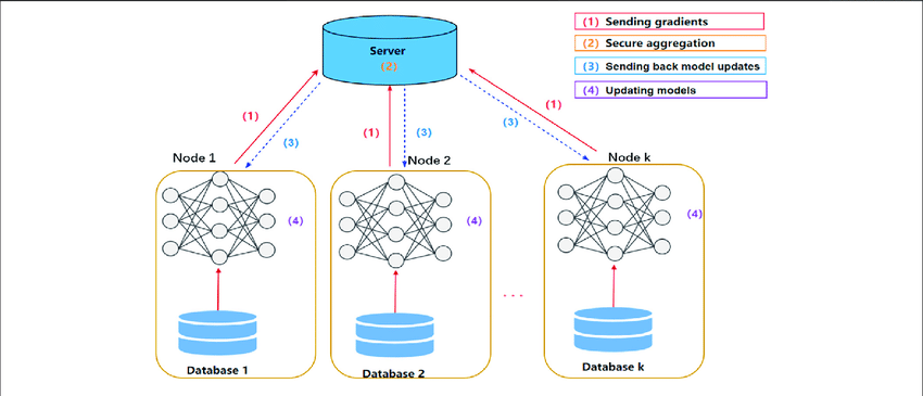
2.3.1 Parameter Server Architecture
A common paradigm in distributed ML.
- Workers compute gradients
- Parameter server (PS) stores global model parameters
- PS updates model and sends new parameters to workers
Advantages:
- Simple architecture
- Scales to many workers
Disadvantages:
- Parameter server can become a bottleneck
- Requires efficient communication strategies
2.3.2 All-Reduce Architecture
No central server.
Workers directly communicate with each other using collective operations like all-reduce.
- Workers sum or average gradients among themselves
- Faster than PS architecture
- Used in high-performance deep learning (e.g., NCCL, Horovod, PyTorch DDP)
2.4 Synchronous vs Asynchronous Training
2.4.1 Synchronous Distributed Training
- All workers compute gradients for their batches
- Aggregator waits until every worker finishes
- Gradients averaged → parameters updated
Pros:
- Stable updates
- Equivalent to large-batch SGD
Cons:
- Straggler problem: slowest worker delays all others
2.4.2 Asynchronous Distributed Training
- Workers send gradients whenever they finish
- Parameter server updates immediately
- No need to wait for slow workers
Pros:
- Faster throughput
- Scales to many workers
Cons:
- “Stale gradients” (gradients computed on old versions of parameters)
- Harder to reason about convergence
2.5 Communication Challenges
Distributed ML performance is often limited by communication, not computation.
Key issues:
- Bandwidth constraints
- High latency between machines
- Gradient size (very large tensors)
- Repeated synchronization overhead
Common solutions:
- Gradient compression
- Quantization (8-bit, 1-bit SGD)
- Sparse updates
- Reducing synchronization frequency
2.6 MapReduce for Machine Learning
MapReduce enables large-scale ML by splitting work into two stages:
Map phase:
- Data is partitioned across workers
- Each worker computes partial results (e.g., cluster assignments, local counts)
Reduce phase:
- Partial results combined
- Final model parameters updated or final statistics computed
Common algorithms adapted to MapReduce:
-means clustering - Naive Bayes classification
- Logistic regression (via iterative MapReduce jobs)
- Linear regression
- Frequent itemset mining
Although slower for iterative algorithms, MapReduce pioneered scalable ML and heavily influenced modern systems like Spark.
2.7 Apache Spark MLlib
Spark MLlib is a distributed ML library built on Resilient Distributed Datasets (RDDs).
Advantages:
- Faster than MapReduce due to in-memory computing
- Supports iterative ML workloads
- Contains scalable implementations of many ML algorithms
MLlib includes:
- Regression
- Classification
- Clustering
- Collaborative filtering
- Dimensionality reduction
Often seen in industry pipelines.
2.8 Fault Tolerance in Distributed ML
Distributed systems must handle machine failures gracefully.
Common techniques:
- Checkpointing: periodically saving model state
- Replication: redundant copies of data/parameters
- Task re-execution: Spark or Hadoop automatically re-runs failed tasks
- Stateless workers: easier to restart after crash
Fault tolerance is crucial because training jobs may run for days.
2.9 Popular Frameworks for Distributed ML
- Apache Hadoop (MapReduce model)
- Apache Spark MLlib
- TensorFlow Distributed Strategy
- PyTorch Distributed Data Parallel (DDP)
- Horovod
- Ray Train
Exam answers only need the names + 1-line explanation.
2.10 Advantages of Distributed Learning
- Can train on massive datasets
- Supports very large models
- Reduces training time from days to hours
- Enables real-time or frequent retraining
- Efficient use of modern cluster/GPU hardware
2.11 Limitations of Distributed Learning
- Communication overhead can dominate computation
- Straggler problem affects speed
- Synchronization complexity
- Requires careful system design
- Fault tolerance increases overhead
- Debugging distributed programs is harder
2.12 Real-World Applications
- Training deep neural networks (vision, NLP, transformers)
- Large-scale recommendation systems (Netflix, YouTube)
- Search ranking models (Google, Bing)
- Ad-click prediction
- Large-scale clustering and topic modelling
- Distributed reinforcement learning
- High-performance scientific computing
3. Semi-Supervised Learning (SSL)
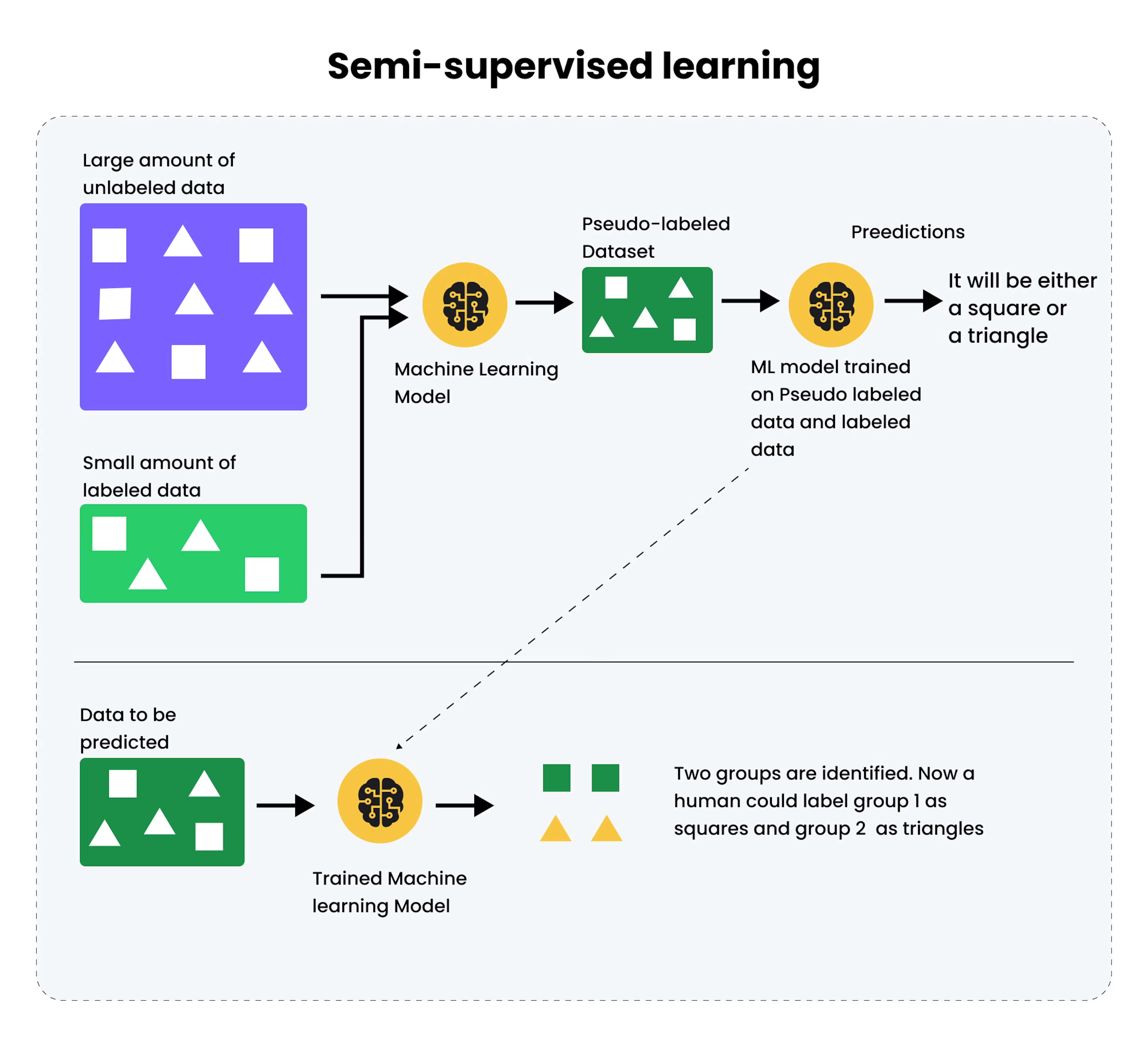
Semi-supervised learning is a machine learning paradigm where a model is trained using a small amount of labeled data together with a large amount of unlabeled data.
It lies between supervised and unsupervised learning and is extremely useful when labeled data is expensive or difficult to obtain, but unlabeled data is plentiful.
3.1 Why Semi-Supervised Learning?
In real-world scenarios:
- Labeled data → costly, requires experts
- Unlabeled data → cheap, extremely abundant
Examples:
- Speech audio recordings
- Millions of images from the internet
- Medical scan images
- Web pages and documents
Semi-supervised learning uses unlabeled data structure to improve accuracy, reduce overfitting, and learn better decision boundaries.
3.2 Core Intuitions Behind SSL
Semi-supervised learning is built on three major assumptions.
These are crucial exam points.
1. Smoothness Assumption
If two samples
2. Cluster Assumption
Data tends to form clusters.
Points in the same cluster probably have the same label.
3. Manifold Assumption
High-dimensional data lies on a lower-dimensional manifold.
Learning the geometry of the manifold helps assign labels.
These assumptions allow unlabeled data to guide supervised learning.
3.3 Categories of Semi-Supervised Learning Methods
SSL techniques fall into several major groups.
3.3.1 Self-Training (Self-Learning)
- Train a supervised model on labeled data
- Use it to predict labels for unlabeled data
- Choose high-confidence predictions
- Add them to training data
- Retrain model
- Repeat until convergence
This is simple but effective for text and image classification.
3.3.2 Co-Training
Proposed by Blum & Mitchell.
Idea:
- Use two different models, each trained on different feature sets (views)
- Each model labels unlabeled data for the other
Works when:
- Data has multiple natural representations
- e.g., web pages: (text content, hyperlinks)
- videos: (audio, video frames)
Co-training improves learning when views are independent.
3.3.3 Semi-Supervised SVMs (Transductive SVMs)
Goal:
Find a decision boundary that not only separates labeled data but also avoids cutting through high-density regions of unlabeled points.
This enforces the cluster assumption.
Optimization attempts to maximize margin while respecting unlabeled data structure.
3.3.4 Graph-Based Semi-Supervised Learning
Construct a graph:
- Nodes = data points
- Edges = similarity weights (e.g., Gaussian kernel)
Labels from labeled nodes are propagated to nearby unlabeled nodes through the graph.
Methods include:
- Label propagation
- Label spreading
- Graph regularization
Graph SSL works well when data has strong cluster/graph structure.
3.3.5 Generative Models
Fit a probability model to both labeled and unlabeled data.
Example: Gaussian Mixture Models (GMMs)
- Fit GMM on all data
- Infer which component likely corresponds to which class
- Use EM algorithm to refine parameters
Generative SSL assumes a model like:
Works only when generative assumptions are valid.
3.3.6 Consistency Regularization Methods (Modern SSL)
Modern deep learning-based SSL techniques enforce:
A model should output similar predictions for perturbed versions of the same input.
Examples:
- Adding noise
- Data augmentation
- Dropout
- Input masking
Used in modern algorithms like:
-Model - Temporal Ensembling
- Mean Teacher
- FixMatch
These methods dominate state-of-the-art SSL performance on images and text.
3.4 Pseudo-Labeling (Important in exams)
A very popular and simple SSL technique:
- Use supervised model to generate pseudo-labels for unlabeled data
- Add pseudo-labeled data to training set
- Retrain
Works extremely well with deep neural networks when unlabeled data is abundant.
3.5 Loss Functions in Semi-Supervised Learning
Most SSL methods combine:
Supervised Loss (from labeled samples)
Unsupervised Loss (from unlabeled samples)
Often based on:
- consistency loss
- entropy minimization
- graph regularization
General combined objective:
Where
3.6 Benefits of Semi-Supervised Learning
- Significantly reduces labeling cost
- Improves accuracy over pure supervised learning
- Uses large-scale unlabeled data efficiently
- Reduces overfitting (unlabeled data constrains decision boundaries)
- Works well in real-world domains where annotations are scarce
3.7 Limitations of SSL
- Wrong pseudo-labels can mislead the model
- Sensitive to assumptions (cluster/smoothness manifold)
- Co-training requires true multiple views
- Graph-based methods scale poorly to large datasets
- Performance depends on data distribution structure
3.8 Real World Applications
- Speech recognition (lots of unlabeled audio)
- Web classification (billions of unlabeled pages)
- Medical imaging (labels need experts)
- Large-scale image classification
- Text classification in NLP
- Video classification
- Biological data analysis
Semi-supervised learning is heavily used in industrial pipelines where labeling is expensive but data availability is massive.
4. Active Learning
Active Learning (AL) is a machine learning approach where the model is allowed to choose which data points should be labeled, with the goal of achieving high accuracy using as few labeled examples as possible.
This is extremely useful when unlabeled data is abundant, but labeling is expensive, requiring human experts.
4.1 Why Active Learning?
Labeling can be costly:
- Medical images need radiologists
- Speech transcripts need linguists
- Legal documents need experts
- Sentiment labels need human review
Active learning minimizes labeling cost by selecting only the most informative samples for annotation.
4.2 The Active Learning Loop
The typical AL pipeline:
- Start with a small labeled dataset
- Train a model
- Use the model to analyze an unlabeled pool
- Select the most informative samples from
- Query a human (oracle) to label them
- Add them to
and retrain - Repeat until performance is sufficient
This iterative process concentrates labeling effort where it matters most.
4.3 Query Strategies in Active Learning
The central idea of AL is the query strategy—how the model chooses which samples to label.
4.3.1 Uncertainty Sampling
The model queries samples where it is least confident.
Common uncertainty measures:
A. Least Confidence
Choose sample with lowest predicted probability for its predicted class:
B. Margin Sampling
Choose sample with smallest difference between top two class probabilities:
C. Entropy-Based Sampling
Choose sample with highest prediction entropy:
Used widely for classification and deep learning.
4.3.2 Query-by-Committee (QBC)
Maintain a committee of models trained on current labeled data.
Process:
- Each model votes on label for an unlabeled sample
- Query the sample where committee disagrees the most
Disagreement measures include:
- Vote entropy
- KL divergence among predictions
QBC works well when multiple hypotheses explain the data.
4.3.3 Expected Model Change
Select samples that would cause the largest change in model parameters if labeled and used for training.
Intuition:
Label points that will significantly improve the model.
4.3.4 Expected Error Reduction
Choose samples expected to reduce future generalization error the most.
This method is theoretically strong but computationally expensive.
4.3.5 Density-Weighted Sampling
Uncertainty alone may pick outliers.
Density-weighted AL considers:
- uncertainty of the sample
- density of the surrounding region
Idea:
Select uncertain samples in high-density regions, avoiding noise/outliers.
4.4 Active Learning Settings
Active learning can be applied in different settings depending on how data is accessed.
4.4.1 Pool-Based Active Learning
Most common setting.
- Large pool of unlabeled data
- Query strategy selects samples from this pool
- Most practical and widely used
4.4.2 Stream-Based Active Learning
Data arrives as a stream.
- For each incoming sample, decide immediately whether to query it
- Useful for real-time systems
Decision often based on uncertainty threshold.
4.4.3 Membership Query Synthesis
The model generates synthetic examples and asks for labels.
Feels like adversarial example generation.
Rare in practice because queries must be human-understandable.
4.5 Active Learning with Deep Learning (Deep AL)
Deep learning + Active Learning requires scalable strategies:
Common approaches:
- Dropout-based uncertainty estimation
- Use Monte Carlo dropout to estimate confidence
- Embedding-based clustering
- Select representative & uncertain samples
- Consistency-based methods
- Leverage semi-supervised learning ideas
- Adversarial Active Learning
- Use adversarial perturbations to find uncertain regions
Deep AL is used in vision, NLP, and medical imaging.
4.6 Stopping Criteria in Active Learning
When to stop querying?
Common criteria:
- Validation accuracy saturates
- Uncertainty in unlabeled pool decreases
- Budget exhausted (common in exams)
- Model confidence stabilizes
- Minimum change in loss between rounds
4.7 Advantages of Active Learning
- Drastically reduces labeling cost
- Improves performance with fewer labeled samples
- Focuses human effort on hardest/most informative cases
- Works well in domains with expert labeling
- Flexible: can be combined with SSL or RL
4.8 Limitations of Active Learning
- Needs a reliable model uncertainty measure
- Uncertainty sampling can pick outliers
- Computationally expensive for large unlabeled pools
- Requires human-in-the-loop systems
- Not always helpful if unlabeled data is not informative
- Deep AL requires careful engineering
4.9 Real-World Applications
- Medical image labeling (MRI, CT, X-Rays)
- Speech recognition (transcription labeling)
- Document classification
- Named Entity Recognition (NER)
- Optical character recognition
- Fraud detection systems
- Autonomous driving (sample selection for labeling)
- Robotics (safe exploration)
Active learning is heavily used in domains where labels are expensive but unlabeled data is plentiful.
5. Reinforcement Learning (RL)
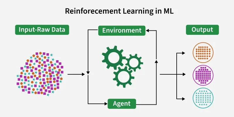
Reinforcement Learning is a learning paradigm where an agent interacts with an environment to achieve a goal. The agent learns by receiving rewards (positive or negative) and tries to maximize the cumulative reward over time by choosing optimal actions.
Unlike supervised learning (has labels) or unsupervised learning (no labels), RL learns from trial and error interactions.
5.1 Core Components of an RL System
Reinforcement Learning problems are formally defined as a Markov Decision Process (MDP).
An MDP consists of:
— State space: all possible environment configurations — Action space: all possible actions the agent can take — Transition probabilities: how actions move the agent — Reward function: immediate reward after taking action — Discount factor: weighs immediate vs future rewards
Goal:
Learn a policy
5.2 Return and Value Functions
Return
Total discounted reward from time
State Value Function
Expected return from state
Action Value Function (Q-value)
These values help the agent decide the best actions.
Upto here the equations are important. After that learning further equations are optional from the exam pov.
5.3 Categories of RL Methods
1. Model-Based RL
- The agent learns a model of the transition dynamics
- Can simulate future states and plan actions (e.g., Dyna-Q)
Useful for:
- planning
- environments with limited interaction opportunities
2. Model-Free RL
The agent learns directly from experience, without learning transition models.
Two main categories:
A. Value-Based Methods
Learn
Examples:
- Q-Learning
- SARSA
- Deep Q-Networks (DQN)
B. Policy-Based Methods
Directly learn policy
Examples:
- REINFORCE
- Actor-Critic methods
- PPO, A2C, DDPG
5.4 Temporal Difference Learning (TD)
TD Learning updates values using bootstrapping:
TD is used in:
- SARSA
- Q-learning
- Actor-critic methods
Key advantage:
- Learns online, step-by-step
- Does not require full trajectories
5.5 Q-Learning (Off-Policy)
Q-learning aims to learn the optimal action-value function
Update rule:
Properties:
- Off-policy: learns from optimal future policy, even if taking exploratory actions
- Converges under certain conditions
Used heavily in:
- games
- robotics
- autonomous navigation
- Minecraft mod RL agents (like yours)
5.6 SARSA (On-Policy)
Update rule:
Difference vs Q-learning:
- SARSA uses the action actually taken
- More conservative
- Safer in risky or stochastic environments
5.7 Deep Q-Learning (DQN)
DQN extends Q-learning using neural networks:
Key innovations that made deep RL succeed:
-
Experience Replay
- Stores
tuples - Samples random minibatches
- Breaks correlation between consecutive samples
- Stores
-
Target Network
- A copy of the Q-network
- Updated slowly
- Stabilizes learning
- A copy of the Q-network
-
Exploration via
-greedy - Take random actions with probability
- Reduces over time
- Take random actions with probability
DQN achievements:
- Solved Atari 2600 games
- Base approach for many modern RL methods
5.8 Policy Gradient Methods
Policy gradients optimize the policy directly.
Objective:
Gradient update:
Advantages:
- Works with continuous actions
- More stable for high-dimensional control
- Avoids Q-value instability
Examples:
- REINFORCE
- DDPG
- PPO
- A3C / A2C
5.9 Actor-Critic Methods
Combine the best of value-based and policy-based methods.
Actor: learns the policy
Critic: learns the value function
Critic guides actor updates, making learning faster and stable.
Used widely in robotics and continuous control.
5.10 Exploration vs Exploitation
Key challenge in RL:
- Exploration → try new actions to discover rewards
- Exploitation → use known best actions
Common strategies:
-greedy - Softmax action selection
- Upper Confidence Bound (UCB)
- Intrinsic motivation (curiosity)
5.11 Reward Engineering
Rewards must be designed carefully to avoid:
- reward hacking
- unintended behaviors
- local optimum traps
Good reward design often makes or breaks real RL agents.
5.12 Challenges in RL
- Sample inefficiency (needs many interactions)
- High variance in learning
- Instability with deep networks
- Sparse rewards
- Safety issues
- Real-world physical risks
- Hard credit assignment problem
5.13 Applications of Reinforcement Learning
- Game agents (Atari, AlphaGo, AlphaZero)
- Robotics (manipulation, navigation)
- Autonomous vehicles
- Recommendation systems
- Industrial control and automation
- Finance & trading agents
- Energy optimization
- Personalized tutoring systems
- Your Minecraft AI mod’s autonomous behavior
RL is used wherever decisions must be learned from interaction rather than labeled examples.
6. Bayesian Learning
Refer to Module 1 -- Supervised Learning -- Machine Learning#3. Naive Bayes Classifier first.
After that:
Variants of Naive Bayes
- Multinomial NB: Models feature counts (e.g., raw word counts). Good for document classification.
- Bernoulli NB: Models binary features (word present / not). Useful when presence matters more than frequency.
- Gaussian NB: For continuous features; assumes
.
Numerical stability (use logs)
Multiply many probabilities leads to underflow. Compute log-probabilities instead:
General smoothing (Lidstone)
where
Practical notes & caveats
- Complement NB often helps with imbalanced text datasets.
- NB can perform well despite correlated features, but strong feature dependencies can reduce accuracy.
- Probabilities from NB may be poorly calibrated; use calibration methods if probabilities are important.
- Use
MultinomialNB,BernoulliNB,GaussianNBin scikit-learn;partial_fitsupports online updates.
Evaluation
Report accuracy, precision, recall and F1 for imbalanced classes. Consider ROC/AUC where applicable.