Matrices -- Module 3 -- Mathematics -IA
Index
- What are Matrices?
- What is a Vector?
- Vector Addition
- Scalar Multiplication
- Quick Recap Other Vector Operations
- Matrix multiplication
- Linear system of equations and how to solve them, methods of solving them
- Linear Independence
- Rank of a matrix
- Methods to find the rank of a matrix
- Cramer's rule
- The Matrix Inversion method.
- Matrix Inversion method (Adjugate matrix version)
What are Matrices?
1. What is a Matrix?
A matrix is a rectangular array of numbers or symbols arranged in rows and columns. For example:
- The matrix above has 2 rows and 3 columns.
- Such a matrix is called a
(read as "2 by 3") matrix.
2. Types of Matrices
a) Row Matrix
A matrix with just one row.
b) Column Matrix
A matrix with just one column.
c) Square Matrix
Number of rows equals number of columns.
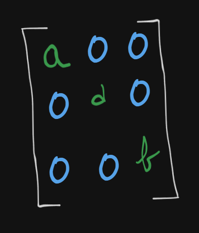
d) Diagonal Matrix
A square matrix where all elements off the main diagonal are zero.
e) Scalar Matrix
A diagonal matrix where all diagonal elements are equal.
f) Identity Matrix (Unit Matrix)
A diagonal matrix with all main diagonal elements equal to 1.
g) Zero Matrix (Null Matrix)
All elements are zero.
3. Matrix Notation
: A matrix named with rows and columns. - Element at row
, column is denoted .
Vectors
What is a Vector?
A vector is an object that has both magnitude (length) and direction. In the context of algebra and matrices, a vector is typically represented as an ordered list of numbers, which can be written as a column or a row. For example, in 3D space:
This is a column vector in
Types of Vectors
- Column vector: Written as an n×1n×1 matrix, like above.
- Row vector: Written as a 1×n1×n matrix, e.g.
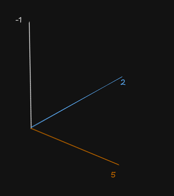
Vector Addition
If you have two vectors of the same size:
Their sum is:
Example:
Geometric interpretation: Scalar multiplication stretches or shrinks the vector, and if the scalar is negative, it reverses its direction.
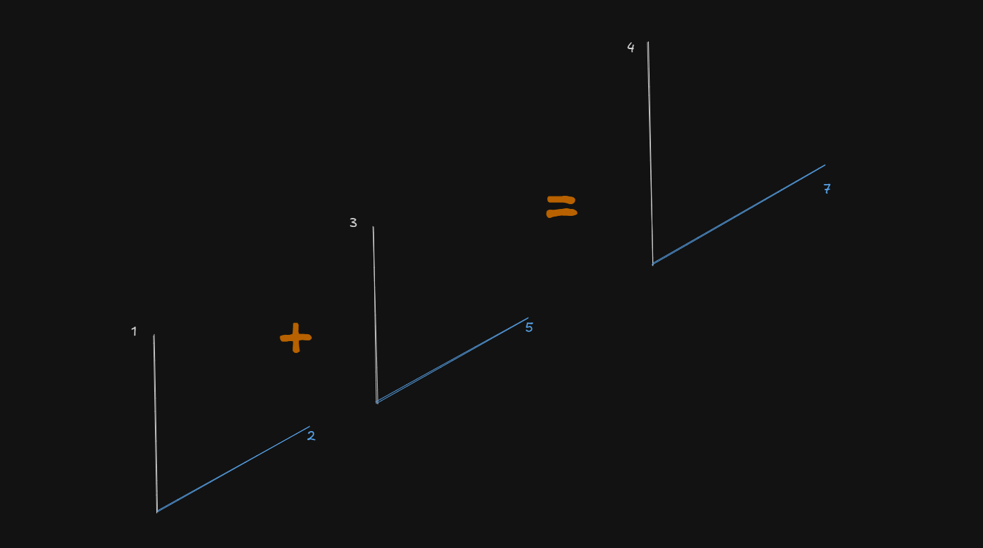
Note the differences in the length of the lines of the vector after addition
Scalar Multiplication
Given a scalar (number)
Example:
Geometric interpretation: Scalar multiplication stretches or shrinks the vector, and if the scalar is negative, it reverses its direction.
Quick Recap: Other Vector Operations
Dot Product (Scalar Product)
Definition:
The dot product of two vectors
It can also be written as:
where
Example 1:
Let
Example 2:
Let:
and
We are asked to find the angle between these two vectors.
Step 1: Compute the dot product
Step 2: Compute the magnitudes
Step 3: Plug into formula to find the angle:
Cross Product(Vector Product)
Definition:
The cross product of two vectors in
The formula is:
Example:
Let
Matrix multiplication
https://www.youtube.com/watch?v=2spTnAiQg4M
What is Matrix Multiplication?
Matrix multiplication is an operation that takes two matrices and produces another matrix. It’s not just multiplying each corresponding entry; instead, you sum the products of rows and columns.
How to verify if the order of multiplication of two matrices is valid or not.
Take these two matrices from the video.
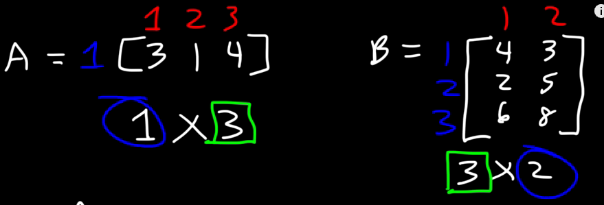
Note how their
If the number of columns of the first matrix, equates to the number of rows of the second matrix, then we can multiply the two matrices.
Which is why
But if you try:
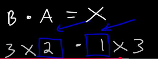
So yes, the order of multiplication of matrices does matter here.
How to Multiply Two Matrices
You can either the watch the video, or read the following here:
Suppose:
The element in the
Or in simple words: dot the
Example
We have to multiply these new matrices.
Let the product matrix be named :
So,
(first row of A and first column of B) (first row of A and second column of B) (second row of A and first column of B) (second row of A and second column of B)
So, the product of the two matrices
Key Properties of Matrix Multiplication
- Not Commutative:
(in general) - Associative:
- Distributive:
- Multiplication by Identity:
, where is the identity matrix
Linear system of equations and how to solve them, methods of solving them
For people like me who are revisiting Semester 1 math after crossing semester 6, you will probably know the content bomb that I am about to drop here from sem 6 notes.
For first timers however, it will still be just as easily understandable to you.
The following content will cover:
- Gaussian Elimination method of solving a system of linear equations
- Gauss-Jordan method of solving a system of linear equations
- Matrix inversion method (using two ways) and using the method of matrix inversion to solve a system of linear equations
- Determinant of a matrix (2x2) and (3x3)
- Transpose of a matrix
By all means, enjoy:
Gaussian Elimination method to find the solution for a system of linear equations
This method converts a system of equations into an upper-triangular form (where all entries below the main diagonal are zero) so that you can then solve for the unknowns via back substitution.
https://www.youtube.com/watch?v=eDb6iugi6Uk
Example 1
So let's say we have this system of linear equations here
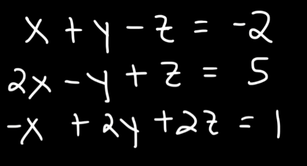
So first of what we will do is construct an augmented matrix using the coefficients of the equations.
Now what we need to do is to convert this to a row-echelon form.
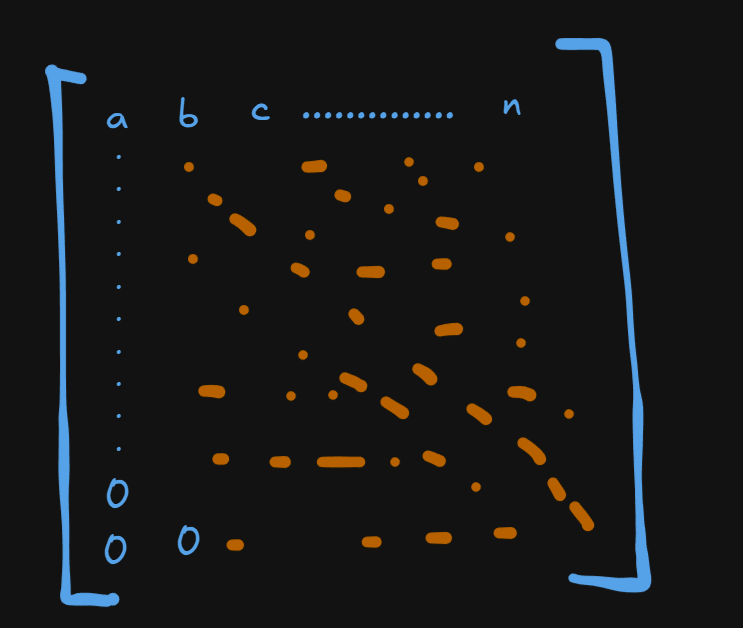
The row-echelon form of this matrix should be something like this :

Note that the bottom left half elements below the diagonal line are all zeroes. (Only works for perfect square matrices)
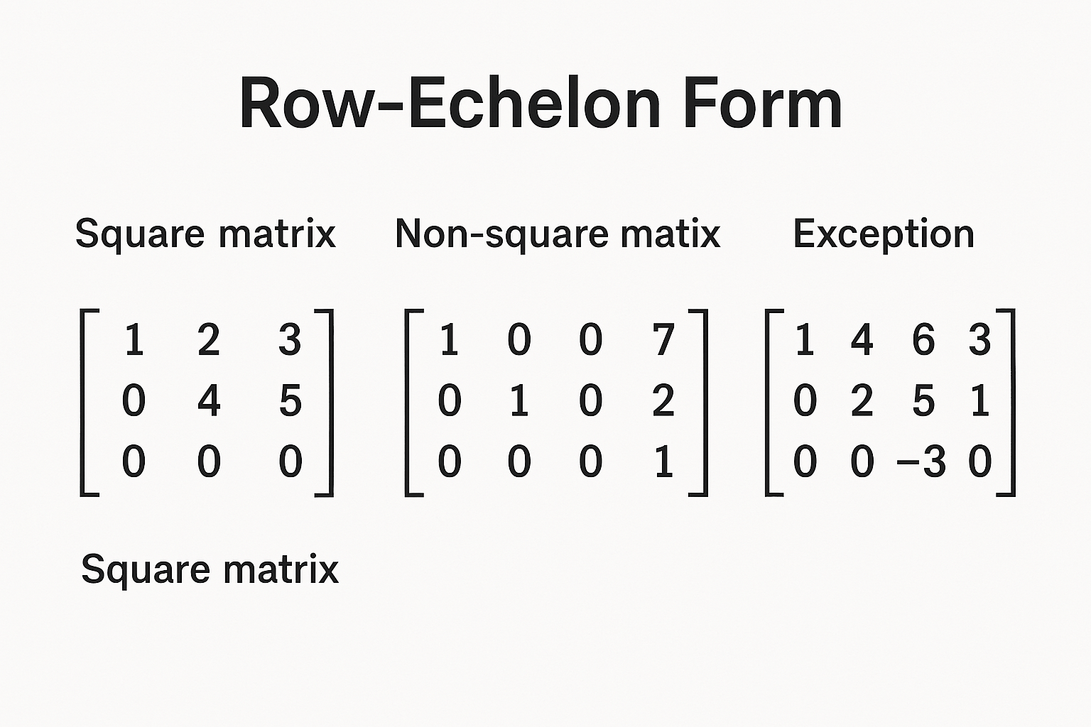
(Image generated by the new version of ChatGPT, not bad indeed.)
So with this matrix, let's call it
How do we convert it to a row-echelon form?
It's done by doing something called a matrix transformation via matrix row operations.
So first of all we select a pivot element. A pivot element is the first non-zero element we encounter in a matrix.
In
Now all our operations will be centered around
So we can do $$R_3 \rightarrow R_1 \ + \ R_3 $$
So the matrix becomes :
Remember that when we add two rows, all elements of the rows are affected.
We can then try :
Then we can do :
We are already there
This can be done by simply for
We have already reached the row-echelon form, but,
We can further simplify the matrix by performing an operation on
Now we can convert the matrix back to equations as :
Now with some simple substitution :
Thus :
Therefore :
So we have the solution for the system of equations as:
Summary:
Always use the format:
where :
For example if we have the rows :
-
Pivot Row (Row 1):
Here, if you want to eliminate the
-variable, the pivot coefficient is 2. -
Target Row (Row 2):
The target coefficient for the
-variable in Row 2 is .****
Example 2
So we can write the matrix as:
Here we will select the pivot element as 2.
So all our operations will be centered around
So to solve remove the coefficients of
So the target row is
So
So $$R_3 \ \to \ R_3 \ - \ m \ \times R_1 \ \implies \ R_3 \ \to \ R_3 \ - \ \frac{2}{2} \ \times R_1 \ \implies R_3 \ - \ R_1$$
So
Therefore the matrix becomes :
Now for Row 2, we have :
Thus Row 2 will be :
Therefore the matrix now becomes :
Now let's remove the
So our pivot component for
But why change pivots now?
The reason is that each pivot is used to clear the entries below it in its column.
The way pivots are chosen are that they are taken from a column which hasn't been used for a pivot, yet.
So :
Therefore
So
Thus,
So the matrix will become :
Now let's convert this matrix back to a system of equations :
So we get :
And finally :
Thus :
Gauss-Jordan Elimination Method
This is similar to the previous method, except here we reduce the matrix even further, to something called a "reduced row echelon form".
https://www.youtube.com/watch?v=eYSASx8_nyg
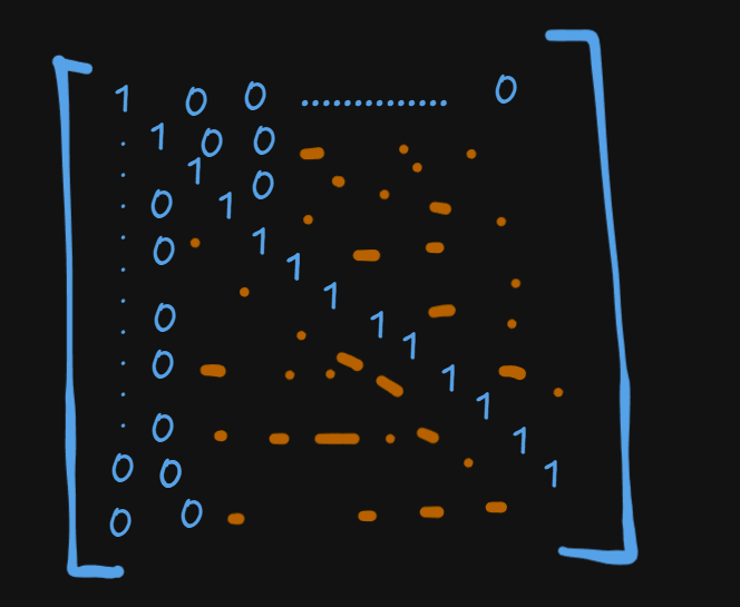
Now this, is the reduced row echelon form.
where
The identity matrix is :

where the diagonal elements of the matrix are 1 and all the other elements are zero.
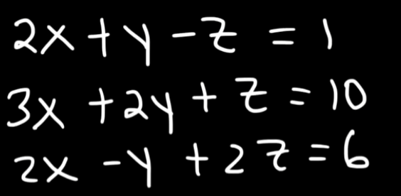
So let's say we have this system of equations here:
We will solve them in the same manner as we did before, only that there will be a few more operations now.
So let's convert this system of equations to an augmented matrix first.
Let's set the pivot element to 1 for the
So the target row is
Thus,
So,
So the matrix becomes :
Now the target is
So:
So the matrix becomes:
Now we set the pivot element to -2 for the
Thus,
So :
So, the matrix now becomes :
Now for the
So:
Note: If we instead tried to set
So,
So, the matrix becomes :
Now for
So :
Thus the matrix becomes :
Now, for the
Forward Elimination vs. Backward Elimination
-
Forward Elimination:
-
Key Point: Once a pivot is chosen in a column, it is used to clear entries downward. You do not worry about entries above because those rows haven't been processed yet.
We did this when we were processing the elements below the diagonal line.
-
-
Backward Elimination (or Back Substitution for RREF):
Once the matrix is in row-echelon form (all entries below each pivot are zero), you perform backward elimination to clear entries above each pivot. This step ensures that each pivot is the only nonzero entry in its column.We are now about to do this with the
component of . -
Why This is Valid:
-
The forward phase ensures that each pivot has zeros below it.
-
The backward phase then uses each pivot to clear above it.
-
Even though the pivot in Row 2 was already used to clear entries below (in Row 3), it must also clear any nonzero entry above it (in Row 1) to satisfy the RREF condition (each pivot column has zeros everywhere except for the pivot itself).
-
-
So we can safely select -2 as the pivot.
So :
Before that we scale
Now
So, proceeding with
So, the final matrix becomes :
Now we can easily convert them back to equations and get the values of
So,
So the solutions are :
The Matrix Inversion method.
Let's walk through the matrix inversion method step by step. The idea is that if you have a system of linear equations in the form
and the coefficient matrix
Pre-requisites before using this method (must) (skip ahead if you already know these).
- Knowing how to find out the determinants of 2x2 and 3x3 matrix. (https://www.youtube.com/watch?v=3ROzG6n4yMc)
- Transpose of a matrix.
- Knowing how to find the inverses of 2x3 and 3x3 matrix. (https://www.youtube.com/watch?v=aiBgjz5xbyg) (2x2) and (https://www.youtube.com/watch?v=Fg7_mv3izR0) (3x3)
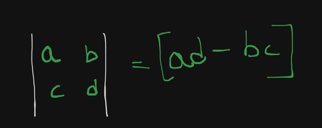
1. The Determinant of a
The determinant of a 2x2 matrix is given by :
Let's say we have this example :
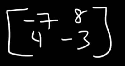
So the determinant of this matrix will be:
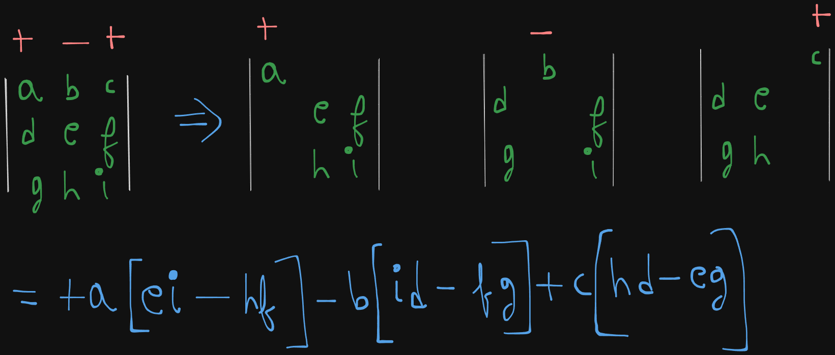
2. Determinant of a
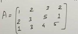
Let's say we have a 3x3 matrix here
The determinant is given by :
which evaluates to :
So let's say we have this example here :
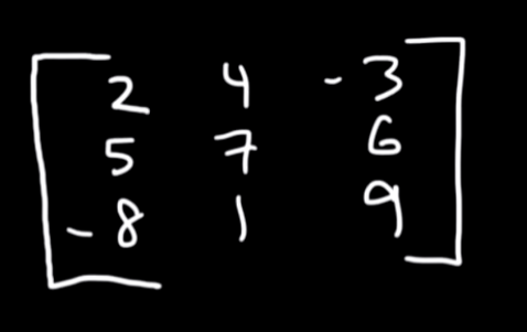
The determinant of this 3x3 matrix will be:
3. Determinant of a
4. Transpose of a matrix.
The transpose of a matrix is just it's rows and columns interchanged.
The transpose of this matrix will be :
Same for a 2x2 matrix :
The transpose will be:
4. Inverse of a 2x2 matrix.
Note: Before trying to invert a matrix, you must first verify if the matrix is invertible or not.
This is done by finding the determinant of the matrix and checking whether it's zero or not.
If the determinant is zero, the matrix is not invertible, else the matrix is invertible.
So if we have a 2x2 matrix
The inverse is given by :
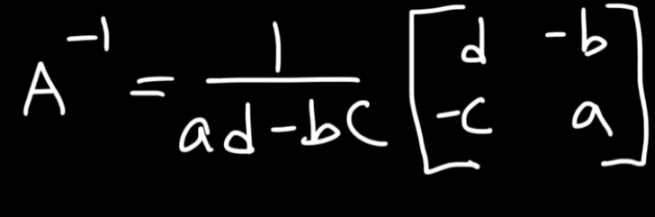
where $$\frac{1}{ad \ - \ bc}$$
is the determinant of the 2x2 matrix.
So let's say we have this matrix example.
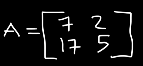
So starting off, let's find the determinant of this matrix.
Now to find the inverse of this matrix :
or
5. Inverse of a 3x3 matrix
Now there are two ways to find the inverse of a 3x3 matrix.
Method 1 : Using Gauss-Jordan Elimination
One way is to use matrix row operations and using the method of Gauss-Jordan elimination to find the inverse of the 3x3 matrix.
https://www.youtube.com/watch?v=Fg7_mv3izR0
So if you have this matrix for example :
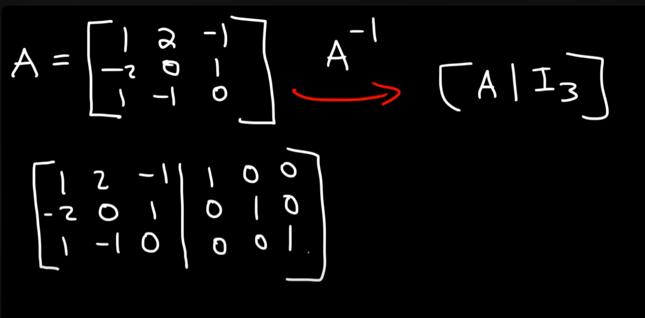
We write it out as in the picture, by augmenting the matrix with the identity matrix.
Then the goal is to perform row operations such that the identity matrix (reduced row echelon form) is on the LHS and on the RHS we get the inverted matrix.
The procedure is the same as Gauss-Jordan elimination, so if you want to see how that's done you can either watch the video in the link or just scroll up to the section of Gauss-Jordan elimination.
Method 2: Using the method of matrix of minors, co-factors and adjugate matrix.
This method is a much less time consuming one that the Gauss-Jordan elimination method.
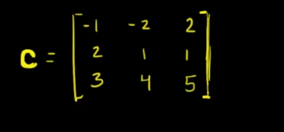
So we start off with a 3x3 matrix
We will create something called a "matrix of minors".
The matrix of minors is of this format:
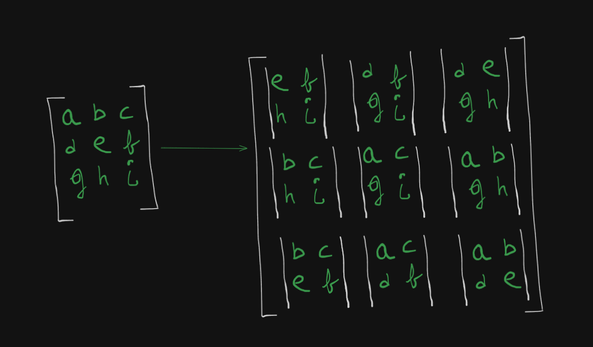
which is basically :
- Choose an element.
- Hide the row and column in which that element is.
- Write the remaining elements in their existing order within a determinant format as singular element of a larger matrix.
- Keep repeating till all the elements in the original matrix, have been chosen.
So with our example matrix it will be :
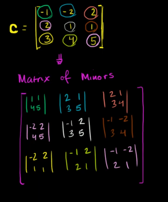
Now after solving the individual determinants :
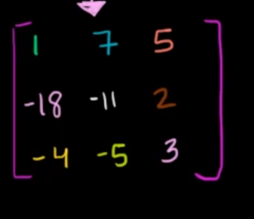
This is the matrix of minors.
Next up is the co-factor matrix.
Simply apply this sign pattern (we see this pattern during the determinant of a 3x3 matrix) :
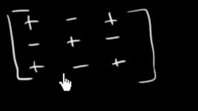
to the elements of the matrix of minors.
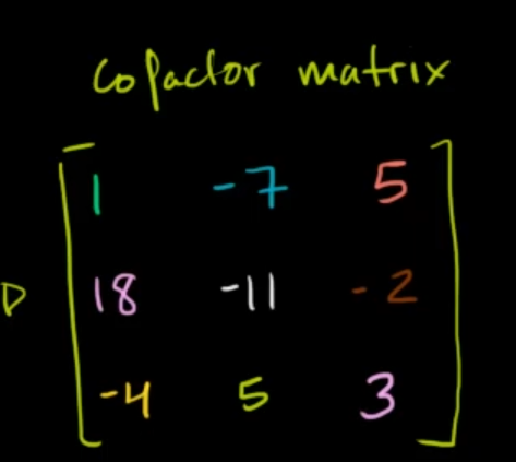
Which now becomes the Co-Factor matrix.
Now we are halfway there!
Next up is the adjugate matrix.
The adjugate matrix is just the transpose of the Co-Factor matrix (rows and columns interchanged).
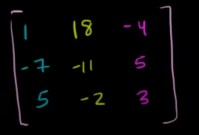
So the final inverse of our 3x3 matrix is the product of the determinant times the adjugate matrix
So we already know how to find the determinant of a 3x3 matrix, so I will be skipping that here
The determinant of this matrix is :
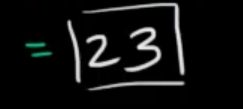
So the final inverse is :
which will result in :
Finding the solution to a system of equations using the matrix inversion method.
So now that we have all the pre-requisites out of the way we can proceed with the matrix inversion method of finding the solution to a system of equations.
Let's proceed with the example we used in the Gauss-Jordan elimination method, better to proceed with a known problem as an example.
So we have the system of equations
So let's convert this system of equations to an augmented matrix first.
However here we will do two things.
We split the augmented matrix into two separate matrices.
One will be the coefficient matrix, let's call it
And the variables matrix, let's call it
And the other one will be the constant matrix, let's call it
Now we need to find :
We will try to invert the coefficient matrix
So let's find out the determinant first:
Since
So I will proceed with the second method here, as it's much faster than doing row operations.
Starting with the matrix of minors :
will be:
(That was quite painful to type and render, but atleast faster than drawing with a mouse).
Now we solve the individual determinants :
So this is the matrix of minors.
Now we apply the sign scheme to get the co-factor matrix:
Now we find the adjugate matrix by transposing the co-factor matrix :
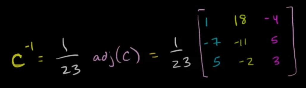
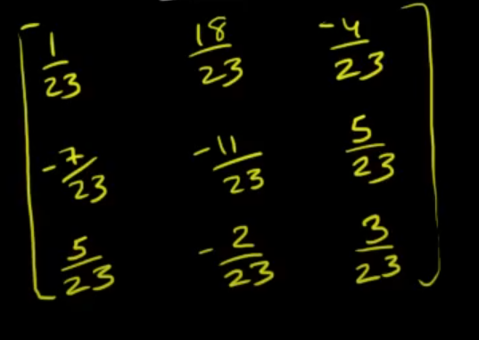
Now we compute the inverse of the matrix :
which will be :
Now using the formula :
we can find out the value of
So :
For
Similarly :
And lastly :
So we get a unique solution this time as :
Simple recap example for the above 3 methods
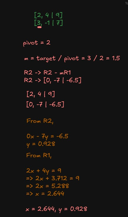
Example
Given a simple
Here's the solution via all 3 methods, Gaussian Elimination, Gauss-Jordan Elimination and Matrix inversion method (Adjugate matrix version)
Gaussian Elimination
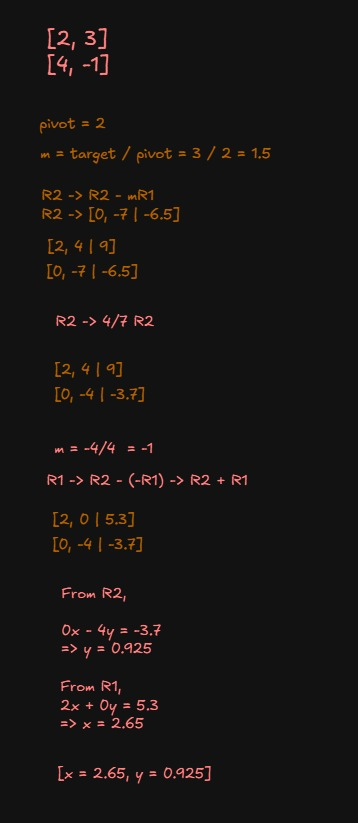
Gauss-Jordan Elimination
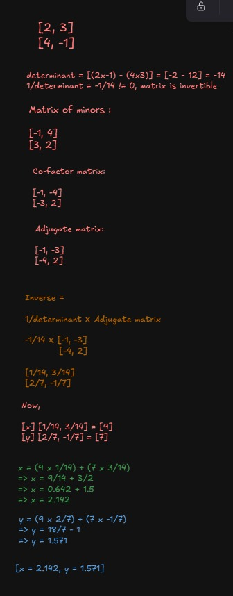
Matrix Inversion method (Adjugate matrix version)
That should clear up any confusions left.
Linear Independence
What is Linear Independence?
Definition:
A set of vectors
is
- If there exists a non-trivial solution (not all
), the vectors are linearly dependent.
Geometric Independence
- In
: Two vectors are linearly independent if they’re not parallel (they don’t lie on the same line through the origin). - In
: Three vectors are linearly independent if they do not all lie in the same plane through the origin.(Point in different axes)
How to Test for Linear Independence (Algebraic Methods)
1. Equation Approach
Write the vector equation:
Set up and solve the corresponding system. If only the trivial solution (
Let's understand this in a little more depth:
What is a Trivial Solution?
When testing if a set of vectors is linearly independent, we ask:
For scalars:
If the only solution is:
then these zeroes are called the trivial solution.
If there exists another set of scalars (not all zero) that solves the above, it’s called a non-trivial solution.
2. Matrix Rank / Row-Reduction
- Form a matrix with the vectors as columns.
- Row-reduce to determine if the only solution to the homogeneous system is the trivial one.
- If the number of pivot columns equals the number of vectors, the set is linearly independent.
3. Determinant Criterion (for Square Matrices) (Easy)
- For
vectors in -dimensional space, place them as columns of an matrix. - If the determinant is non-zero, they’re linearly independent.
Example
Case 1: Linearly Dependent Vectors
Let:
To check independence, solve:
Write them as a system of linear equations:
Solve them however you want.
Now, if we set
Then from the first equation,
So, for any
Not both are always zero (unless
These vectors are linearly dependent.
(Geometrically: they point in the same direction; one is a multiple of the other. (So they are parallel to each other as well))
Case 2: Linearly Independent Vectors
Let,
Solve:
So,
The only solution is
These vectors are linearly independent.
(Geometrically: they point along different axes.)
Rank of a matrix
What is the Rank of a Matrix?
Definition:
The rank of a matrix is the maximum number of linearly independent rows or columns in the matrix.
- It tells you the dimension of the row space or column space (both are equal!).
- In terms of systems of equations, it’s the number of pivots (leading 1’s) you get on reducing a matrix.
How to Find the Rank
1. Row Reduction (Echelon Form)
- Transform the matrix into row-echelon form or reduced row-echelon form (using Gaussian or Gauss-Jordan elimination).
- The rank is the number of non-zero rows (pivots).
2. Largest Non-Zero Minor
- Find the largest square submatrix with a non-zero determinant.
- The size of this submatrix equals the rank.
- Or, in simple terms, just count the number of non-zero rows
Methods to find the rank of a matrix
1. By Normal form
https://www.youtube.com/watch?v=kaphHRq39JI&list=PLF-vWhgiaXWPZ7Ogw6zIZMg4aqUXEwrnJ&index=3
Let's use the given matrix in the example.
Yes, now we are dealing with non-square matrices.
Using normal form you can either use:
- Row-echelon form
- Reduced-row echelon form
And then count the number of non-zero rows to get the rank of the matrix.
Remember that
- In row-echelon form, for the matrix of any
, it's achieved when you have a lower-left triangle of zeroes.
- In reduced-row echelon form, it would look like this:
It is an identity matrix in the case of square matrices.
For non-square matrices:
However it is important to note that:
When solving equations, you do not always get an identity on the diagonal—RREF simply ensures all pivots are 1 and alone in their column. The rest of the structure depends on the rank and shape of the matrix.
IMPORTANT NOTE ON HOW TO DECIDE THAT THE REF or RREF has been reached in a non-square matrix.
Key properties of the Row-Echelon Form
What is a Pivot?
A bit late in the proper clarification definition, but here we go:
A pivot is the first nonzero entry from the left in a row (when moving left to right).
For example:
Row 1: [ 0 0 5 7 ] Pivot is 5
Now,
-
In each nonzero row, the pivot appears to the right (further along in the row) than the pivot in the row above.
-
For example:
- Row 1:
[ 1 * * ](pivot in position 1) - Row 2:
[ 0 1 * ](pivot in position 2 — to the right of the previous row’s pivot) - Row 3:
[ 0 0 1 ](pivot in position 3 — to the right again)
- Row 1:
-
-
All entries below a pivot are zero.
When you find that the all the entries below the pivot in the pivot column are zero, you reach the Row-Echelon Form
For RREF in non-square matrices
Where:
- Pivots are in columns 1 and 2.
- All entries below and above the pivots are zero within those columns.
- Zeros appear at the bottom as necessary.
Example:
Suppose, we have this matrix.
Now, we have to find the rank of a matrix:
Method 1: By Normal Form:
We can either use Gaussian Elimination or Gauss-Jordan Elimination to get the rank.
So, let's use Gaussian Elimination for this.
For
For
For
And now, we have achieved the row-echelon form, so we can stop here.
Judging by the number of non-zero rows, the rank of this matrix is 2.
Let's test now if the Gauss-Jordan elimination results in the same answer or not.
Continuing from the matrix,
For
So, $$R_1 \ \rightarrow \ R_1 \ - \ 3R_3$$
And for
So,
This is an acceptable RREF form, and the number of non-zero rows is 2, so the rank of this matrix is 2.
Method 2: By PAQ form.
You can still watch this video if you need extra clarity, but the explanation there is slightly confusing in my opinion.
https://www.youtube.com/watch?v=bVjjQXnVQ6U&list=PLF-vWhgiaXWPZ7Ogw6zIZMg4aqUXEwrnJ&index=4
This is easy, you just have to convert the matrix to an identity matrix, and then find out the rank by calculating the number of non-zero rows.
We can proceed the same till RREF to get:
Now, to get the identity matrix, just swap
To get the identity matrix.
And this is the PAQ form. The rank is achieved by counting the number of non-zero rows, which in this case is 2, so the rank of the matrix is 2.
Method 3: By Definition of Rank.
https://www.youtube.com/watch?v=-9jSv_F9Hz0&list=PLF-vWhgiaXWPZ7Ogw6zIZMg4aqUXEwrnJ&index=6
Note: This method is only for square matrices.
Steps:
1. Check if the determinant of the largest possible square matrix is non-zero
- If the matrix is square (
), calculate . - If
, the rank = n.
2. If the determinant is zero, check all (n-1)×(n-1) square submatrices
- For each possible square submatrix of size
, find the determinant. - If any one has a non-zero determinant, the rank =
.
3. If all these are zero, check all (n-2)×(n-2) submatrices
- Among all possible submatrices of size
, if any determinant is non-zero, the rank = .
4. Continue down to 1×1 submatrices (individual entries)
- If all minors of order 2 are zero, but at least one entry of the matrix is not zero, the rank = 1.
- If all entries are zero, the rank = 0.
Example
Just follow the example matrix as shown in the video here:
https://www.youtube.com/watch?v=-9jSv_F9Hz0&list=PLF-vWhgiaXWPZ7Ogw6zIZMg4aqUXEwrnJ&index=6
Cramer's rule
What is Cramer’s Rule?
https://www.youtube.com/watch?v=vXqlIOX2itM (2x2 matrix)
https://www.youtube.com/watch?v=Ot87qLTODdQ (3x3 matrix)
Cramer’s Rule provides a solution to a system of
System:
where
is an co-efficient matrix is a vector of variables is a vector of constants
Formula:
For each variable
where:
is the coefficient matrix matrix with the column replaced by must be (system has a unique solution)
Example
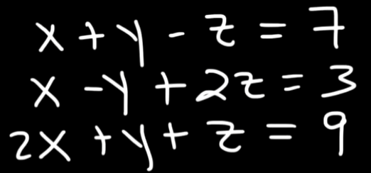
Solve:
Step 1:
Write as
Step 2:
Compute the determinant of A
Since
Step 3: Compute the determinants by swapping both the columns of
(replace 1st column with ) :
(replace the 2nd column with ) :
Step 4: Compute Variables
When Can You Use Cramer’s Rule?
- Number of equations = number of unknowns (square matrix)
(unique solution)