Module 5 -- Vector Spaces -- Continued

Index

Eigenvalues and Eigenvectors
The Cayley-Hamilton Theorem
Symmetric matrices
Diagonalization of matrices (symmetric matrices)
Orthogonal Matrix
Gram-Schmidt Orthogonalization

Eigenvalues and Eigenvectors

https://www.youtube.com/watch?v=PFDu9oVAE-g (must watch this)

Given a square matrix, $A$ , an eigenvector is a non-zero vector $v$ such that:

A v = λ v

where $λ$ is the corresponding eigenvalue.

In words:

An eigenvector of $A$ is a direction that $A$ simply stretches or compresses (by the factor $λ$ ), but does not rotate or mix with other directions.

Breakdown of the Equation

$v \neq 0$ : the vector should not be the zero vector
$λ$ can be positive/negative/zero/complex
All vectors that satisfy this are eigenvectors for eigenvalue $λ$ .

How to find Eigenvalues and Eigenvectors

Step 1: The Characteristic polynomial

Rewriting:

A v = λ v ⟹ (A - λ I) v = 0

Nontrivial solutions ( $v \neq 0$ ) exist only when:

det (A - λ I) = 0

This is called the characteristic equation.

The solutions $λ$ are eigenvalues.

Step 2: Find Eigenvectors

For each eigenvalue $λ$ found above:

Solve ( $A - λ I$ ) $v = 0$
The set of all such nonzero vectors $v$ is the eigenspace for eigenvalue $λ$ .

Detailed Example

Let's use :

A = [\begin{array}{ccc} 2 & 1 \\ 1 & 2 \end{array}]

Step 1: Find the eigenvalues

https://www.youtube.com/watch?v=e50Bj7jn9IQ (This is a video showing a quick trick for calculating eigenvalues, since the more bigger a matrix is, the more complex the equations will be, might get harder to solve.)

We can get that from the characteristic equation :

det (A - λ I) = 0

First:

A - λ I

[\begin{array}{ccc} 2 & 1 \\ 1 & 2 \end{array}] - λ [\begin{array}{ccc} 1 & 0 \\ 0 & 1 \end{array}]

= [\begin{array}{ccc} 2 & 1 \\ 1 & 2 \end{array}] - [\begin{array}{ccc} λ & 0 \\ 0 & λ \end{array}]

= [\begin{array}{ccc} 2 - λ & 1 \\ 1 & 2 - λ \end{array}]

Now,

det (A - λ I)

| \begin{matrix} 2 - λ & 1 \\ 1 & 2 - λ \end{matrix} |

= (2 - λ)^{2} - 1

= (4 - 4 λ + λ^{2}) - 1

= λ^{2} - 4 λ + 3

Now we equate that to zero.

det (A - λ I) = 0

λ^{2} - 4 λ + 3 = 0

And after doing some basic factorization:

(λ - 3) (λ - 1) = 0

So the eigenvalues are:

λ_{1} = 3, λ_{2} = 1

Step 2: Find eigenvectors for each eigenvalue

From the equation:

A - λ I

For $λ_{1} = 3$ ,

⟹ [\begin{array}{ccc} 2 - λ & 1 \\ 1 & 2 - λ \end{array}] = [\begin{array}{ccc} 2 - 3 & 1 \\ 1 & 2 - 3 \end{array}] = [\begin{array}{ccc} - 1 & 1 \\ 1 & - 1 \end{array}]

Now we equate the rows and columns to a vector $v$ where:

v = [\begin{array}{ccc} x \\ y \end{array}]

Applying to both the rows, we get two equations:

- x + y = 0

x - y = 0

From the first equation:

y = x

And from the second equation:

x = y

So all vectors are of the form:

v = [\begin{array}{ccc} 1 \\ 1 \end{array}]

(or any scalar multiple) are eigenvectors with eigenvalue $λ = 3$

Now, for $λ = 1$

⟹ [\begin{array}{ccc} 2 - λ & 1 \\ 1 & 2 - λ \end{array}] = [\begin{array}{ccc} 2 - 1 & 1 \\ 1 & 2 - 1 \end{array}] = [\begin{array}{ccc} 1 & 1 \\ 1 & 1 \end{array}]

So from either row we get the equation:

x + y = 0

So,

x = - y

So, all vectors of the form:

v = [\begin{array}{ccc} 1 \\ - 1 \end{array}]

(or any scalar multiple) are eigenvectors with eigenvalue $λ = 1$

Why Are Eigenvectors and Eigenvalues Important?

Reveal the “axes” along which $A$ acts in the simplest way.
Used in diagonalization, stability analysis, differential equations, quantum mechanics, Google’s PageRank, machine learning and more.

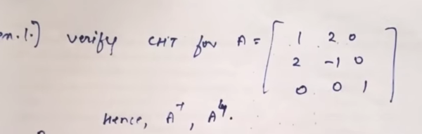
The Cayley-Hamilton Theorem

https://www.youtube.com/watch?v=TNxmupelc-4&list=PLF-vWhgiaXWPZ7Ogw6zIZMg4aqUXEwrnJ&index=9 (must watch)

What is the Cayley-Hamilton Theorem?

Every square matrix A satisfies its own characteristic polynomial $p A (λ) = det (λ I - A)$ .
If $p A (λ) = λ^{n} + c_{n - 1} λ^{n - 1} + \dots + c_{1} λ + c_{0}$ , then
$p A (A) = A^{n} + c_{n - 1} A^{n - 1} + \dots + c_{1} A + c_{0} I = 0$ (the zero matrix).

Or, in very very simple terms,

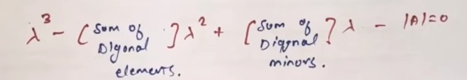
For a given matrix $A_{n \times n}$ , we have to prove that:

(A - λ I) = 0

which is often called the characteristic equation.

Example

Let's use the one given in the video.

Pasted image 20250810132922.png

Given matrix:

A = [\begin{array}{ccc} 1 & 2 & 0 \\ 2 & - 1 & 0 \\ 0 & 0 & 1 \end{array}]

Now, there are two ways to go about this.

Step 1: Write the characteristic equation:

A - λ I = 0

Method 1: We find the eigenvalues, substitute them back into the characteristic equation's LHS and then find out if it equates to the RHS.

Method 2: We follow the steps given in the video.

Let's try method 1.

Step 2: Find the eigenvalues

[\begin{array}{ccc} 1 & 2 & 0 \\ 2 & - 1 & 0 \\ 0 & 0 & 1 \end{array}] - [\begin{array}{ccc} λ & 0 & 0 \\ 0 & λ & 0 \\ 0 & 0 & λ \end{array}]

[\begin{array}{ccc} 1 - λ & 2 & 0 \\ 2 & - 1 - λ & 0 \\ 0 & 0 & 1 - λ \end{array}]

Now, find the determinant of this matrix:

= (1 - λ) [(- 1 + λ - λ + λ^{2}] - 2 [2 - 2 λ - 0] + 0

= (1 - λ) [- 1 + λ^{2}] - [4 - 4 λ]

⟹ - 1 + λ^{2} + λ - λ^{3} - 4 + 4 λ = 0

⟹ - λ^{3} + λ^{2} + 5 λ - 5 = 0

Now it is gonna be a massive pain to solve this equation and find the damn roots.

And I am not kidding about this.

Skip ahead to Let's use the given roots to see if method 1 works in theory or not. to see if this approach pans out or not, and then I will show the easy approach to continue from once we have found the equation (from the video, method 2)

Here's what a search on perplexity did, a massive rabbit hole.

Perplexity(GPT 4.1)'s solution for the cubic equation.

Ah yes now I caught the sign mistake, lamda^3 should have a negative sign. Now then that we have this equation, what would be it's roots?

(I had previously made an error in the sign for $λ^{3}$ which I spent 30 minutes debugging since I skipped a lot of the math and did it in my head, retracing the steps manually took time)

Great! Now that we have the correct characteristic equation:

λ^{3} - λ^{2} - 5 λ + 5 = 0

Let's find its roots.

Analytical Approach

This cubic is not easily factorable with integers, so let's look for rational roots using the Rational Root Theorem:

Possible rational roots: $\pm 1, \pm 5$ (factors of 5 over 1).

Try $λ = 1$ : $1 - 1 - 5 + 5 = 0$
So, $λ = 1$ is a root!

Now divide the cubic by $(λ - 1)$ :

Synthetic Division

Divide $λ^{3} - λ^{2} - 5 λ + 5$ by $(λ - 1)$ :

So, quotient is: $λ^{2} - 5$ .

Therefore:

λ^{3} - λ^{2} - 5 λ + 5 = (λ - 1) (λ^{2} - 5)

Roots of the Quadratic

λ^{2} - 5 = 0 ⟹ λ = \pm \sqrt{5}

Final Roots

\begin{aligned} λ_{1} & = 1 \\ λ_{2} & = \sqrt{5} \approx 2.236 \\ λ_{3} & = - \sqrt{5} \approx - 2.236 \end{aligned}

Let's use the given roots to see if method 1 works in theory or not.

So we have the roots as:

\begin{aligned} λ_{1} & = 1 \\ λ_{2} & = \sqrt{5} \approx 2.236 \\ λ_{3} & = - \sqrt{5} \approx - 2.236 \end{aligned}

which are the eigenvalues.

The CHT says that:

For a given matrix $A_{n \times n}$ , we have to prove that:

(A - λ I) = 0

or it should result in a $3 \times 3$ null matrix:

[\begin{array}{ccc} 0 & 0 & 0 \\ 0 & 0 & 0 \\ 0 & 0 & 0 \end{array}]

However, unfortunately that's not the case, as you will see below.

Applying into equation:

A - λ I

For $λ_{1} = 1$

[\begin{array}{ccc} 1 & 2 & 0 \\ 2 & - 1 & 0 \\ 0 & 0 & 1 \end{array}] - [\begin{array}{ccc} 1 & 0 & 0 \\ 0 & 1 & 0 \\ 0 & 0 & 1 \end{array}] = [\begin{array}{ccc} 0 & 2 & 0 \\ 2 & - 2 & 0 \\ 0 & 0 & 0 \end{array}]

which unfortunately is not the null matrix.

For $λ_{2} = 2.236$

[\begin{array}{ccc} 1 & 2 & 0 \\ 2 & - 1 & 0 \\ 0 & 0 & 1 \end{array}] - [\begin{array}{ccc} 2.236 & 0 & 0 \\ 0 & 2.236 & 0 \\ 0 & 0 & 2.236 \end{array}] = [\begin{array}{ccc} - 1.236 & 2 & 0 \\ 2 & - 3.236 & 0 \\ 0 & 0 & - 1.236 \end{array}]

which also, again, is not the null matrix.

For $λ_{3} = - 2.236$

[\begin{array}{ccc} 1 & 2 & 0 \\ 2 & - 1 & 0 \\ 0 & 0 & 1 \end{array}] - [\begin{array}{ccc} - 2.236 & 0 & 0 \\ 0 & - 2.236 & 0 \\ 0 & 0 & - 2.236 \end{array}] = [\begin{array}{ccc} 3.236 & 2 & 0 \\ 2 & 1.236 & 0 \\ 0 & 0 & 3.236 \end{array}]

which also, again, is not the null matrix.

Key takeaway?

Sure the roots didn't pan out. But:

We don't have to use this method from the video:

Pasted image 20250810143500.png

which will lead into all sorts of messes to find out the equation of:

- λ^{3} + λ^{2} + 5 λ - 5 = 0

which is almost the same in the video:

Pasted image 20250810143622.png

that we can just achieve if we multiply both sides by -1

λ^{3} - λ^{2} - 5 λ + 5 = 0

But, for continuity's sake, let's not do that and continue with our previously achieved equation:

- λ^{3} + λ^{2} + 5 λ - 5 = 0

Remember the end goal here is to check if:

A - λ I

equates to zero or not.

So, how do we proceed after this?

We just replace $λ$ with the matrix $A$ .

from the equation:

- λ^{3} + λ^{2} + 5 λ - 5 = 0

which is derived from:

A - λ I

So the equation becomes:

- A^{3} + A^{2} + 5 A - 5 = 0

Now we verify the LHS part only to see if it equates to zero or not.

Also we must add a tweak:

- A^{3} + A^{2} + 5 A - 5 I = 0

since we are replacing the eigenvalues with entire matrices, every term must be on the same size of the replacement matrix.

Since the last term was just a constant, we can write $5 = 5 \times 1 = 5 \times I$ , where $I$ is the corresponding identity matrix.

Why did we do this?

A scalar like 5 cannot be added to or subtracted from a matrix; the objects must be conformable. The identity matrix I acts as the multiplicative identity for matrices, so the constant term is represented as 5I (a matrix with 5 on the diagonal and 0 elsewhere). This way every term is a 3×3 matrix and they can be summed.

So,

- A^{3} + A^{2} + 5 A - 5 I

{[\begin{array}{ccc} 1 & 2 & 0 \\ 2 & - 1 & 0 \\ 0 & 0 & 1 \end{array}]}^{3} + {[\begin{array}{ccc} 1 & 2 & 0 \\ 2 & - 1 & 0 \\ 0 & 0 & 1 \end{array}]}^{2} + 5 [\begin{array}{ccc} 1 & 2 & 0 \\ 2 & - 1 & 0 \\ 0 & 0 & 1 \end{array}] - 5 [\begin{array}{ccc} 1 & 0 & 0 \\ 0 & 1 & 0 \\ 0 & 0 & 1 \end{array}]

Welp, the matrix multiplication is gonna be a pain lol.

So,:

A^{2} = [\begin{array}{ccc} 1 & 2 & 0 \\ 2 & - 1 & 0 \\ 0 & 0 & 1 \end{array}] \times [\begin{array}{ccc} 1 & 2 & 0 \\ 2 & - 1 & 0 \\ 0 & 0 & 1 \end{array}]

⟹ [\begin{array}{ccc} (1 \times 1 + 2 \times 2 + 0) & (1 \times 2 + 2 \times - 1 + 0) & (0 + 0 + 0) \\ (2 \times 1 + - 1 \times 2 + 0) & (2 \times 2 + - 1 \times - 1 + 0) & (0 + 0 + 0) \\ (0 + 0 + 0) & (0 + 0 + 0) & (0 + 0 + 1) \end{array}]

= [\begin{array}{ccc} 5 & 0 & 0 \\ 0 & 5 & 0 \\ 0 & 0 & 1 \end{array}]

Now,

A^{3} = [\begin{array}{ccc} 1 & 2 & 0 \\ 2 & - 1 & 0 \\ 0 & 0 & 1 \end{array}] \times A^{2} = [\begin{array}{ccc} 5 & 0 & 0 \\ 0 & 5 & 0 \\ 0 & 0 & 1 \end{array}]

⟹ [\begin{array}{ccc} (1 \times 5 + 0 + 0) & (0 + 2 \times 5 + 0) & (0 + 0 + 0) \\ (2 \times 5 + 0 + 0) & (0 + - 1 \times 5 + 0) & (0 + 0 + 0) \\ (0 + 0 + 0) & (0 + 0 + 0) & (0 + 0 + 1) \end{array}]

= [\begin{array}{ccc} 5 & 10 & 0 \\ 10 & - 5 & 0 \\ 0 & 0 & 1 \end{array}]

And lastly,

5 A = 5 \times [\begin{array}{ccc} 1 & 2 & 0 \\ 2 & - 1 & 0 \\ 0 & 0 & 1 \end{array}]

= [\begin{array}{ccc} 5 & 10 & 0 \\ 10 & - 5 & 0 \\ 0 & 0 & 5 \end{array}]

and:

5 I = [\begin{array}{ccc} 5 & 0 & 0 \\ 0 & 5 & 0 \\ 0 & 0 & 5 \end{array}]

Finally arranging them all together:

- [\begin{array}{ccc} 5 & 10 & 0 \\ 10 & - 5 & 0 \\ 0 & 0 & 1 \end{array}] + [\begin{array}{ccc} 5 & 0 & 0 \\ 0 & 5 & 0 \\ 0 & 0 & 1 \end{array}] + [\begin{array}{ccc} 5 & 10 & 0 \\ 10 & - 5 & 0 \\ 0 & 0 & 5 \end{array}] - [\begin{array}{ccc} 5 & 0 & 0 \\ 0 & 5 & 0 \\ 0 & 0 & 5 \end{array}]

= [\begin{array}{ccc} 0 & 0 & 0 \\ 0 & 0 & 0 \\ 0 & 0 & 0 \end{array}]

which is now, the null matrix or zero matrix.

Thus:

A - λ I = 0

or for a better statement:

p (A) = - λ^{3} + λ^{2} + 5 λ - 5 = 0

is proved, which verifies the Cayley-Hamilton Theorem for this matrix.

Symmetric matrices

https://www.youtube.com/watch?v=vSczTbgc8Rc (watch the first two halves of the video to understand all about symmetric matrices)

Definition and basic properties

A real matrix $A \in R^{n \times n}$ is symmetric if $A = A^{T}$ , where $T$ is the transpose of $A$
Entries mirror across the main diagonal: $a_{i j} = a_{j i}$ .
Symmetric matrices are always diagonalizable over R and have real eigenvalues.
Their eigenvectors are orthogonal i.e. perpendicular to each other.

Pasted image 20250814185919.png

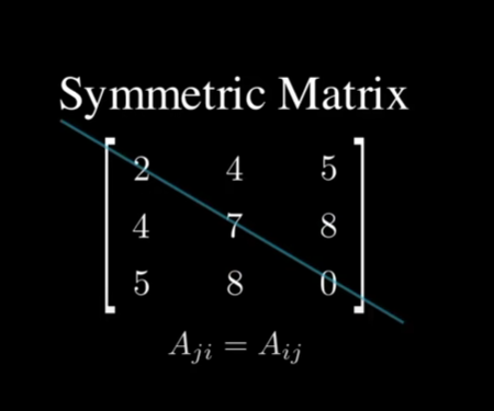
See how the elements on both sides of the diagonal, except the starting and ending element are the same? These are called symmetric matrices.

Diagonalization of matrices (symmetric matrices)

https://www.youtube.com/watch?v=sikqqbbJUXc&list=PLF-vWhgiaXWPZ7Ogw6zIZMg4aqUXEwrnJ&index=13

For a matrix $A$ , it's diagonalized version can be obtained by using this formula:

D = M^{- 1} A M

where:

$M$ is the modal matrix, which is obtained as follows:

Write the characteristic equation $det (A - λ I) = 0$
Solve L.H.S to get a characteristic equation of type $λ^{3} \pm a λ^{2} \pm b λ \pm c$
Instead of replacing $λ$ with $A$ , solve the equation to find the roots i.e. the eigenvalues. (Refer to previous sections)
Substitute the eigenvalues in the derived equation to get the eigenvectors in form of:

x_{1} = [\begin{array}{ccc} a_{1} \\ b_{1} \\ c_{1} \end{array}]

x_{2} = [\begin{array}{ccc} a_{2} \\ b_{2} \\ c_{2} \end{array}]

x_{3} = [\begin{array}{ccc} a_{3} \\ b_{3} \\ c_{3} \end{array}]

Now, the modal matrix $M$ is achieved by:

M = [\begin{array}{ccc} [\begin{array}{ccc} a_{1} \\ b_{1} \\ c_{1} \end{array}] & [\begin{array}{ccc} a_{2} \\ b_{2} \\ c_{2} \end{array}] & [\begin{array}{ccc} a_{3} \\ b_{3} \\ c_{3} \end{array}] \end{array}]

By writing each eigenvector as the column vectors of the modal matrix.

Then we can calculate the inverse, plug them in the formula, and after doing the math :

We should get a matrix like this

D = [\begin{array}{ccc} a & 0 & 0 \\ 0 & b & 0 \\ 0 & 0 & c \end{array}]

which is the diagonal matrix. If we don't get this matrix, then it means the given matrix is not diagonalizable.

Example

For example please refer to the examples in the video :

https://www.youtube.com/watch?v=sikqqbbJUXc&list=PLF-vWhgiaXWPZ7Ogw6zIZMg4aqUXEwrnJ&index=13

Orthogonal Matrix

https://www.youtube.com/watch?v=wciU07gPqUE&t=117s (watch this part)

An orthogonal matrix is basically a matrix whose column vectors are orthogonal (perpendicular to each other), and also their dot product would equate to zero.

Pasted image 20250817135734.png

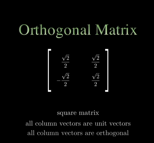
And the column vector's length is always one, hence they are unit vectors.

For example if we take the column vector:

[\begin{array}{ccc} \frac{\sqrt{2}}{2} \\ - \frac{\sqrt{2}}{2} \end{array}]

we can find the length of this column vector by taking the square root of the sum of the squares of the elements:

\sqrt{(\frac{\sqrt{2}}{2})^{2} + (- \frac{\sqrt{2}}{2})^{2}} = \sqrt{(\frac{2}{4}) + (\frac{2}{4})} = \sqrt{\frac{1}{2} + \frac{1}{2}} = \sqrt{1} = 1

Same goes for the other column vector, which means these are unit vectors.

Gram-Schmidt Orthogonalization

https://www.youtube.com/watch?v=UOZjINOGLog (must watch)

https://www.youtube.com/watch?v=rHonltF77zI (another way to visualize this)

https://www.youtube.com/watch?v=tu1GPtfsQ7M (example of method 2)

Index

Eigenvalues and Eigenvectors

Breakdown of the Equation

How to find Eigenvalues and Eigenvectors

Step 1: The Characteristic polynomial

Step 2: Find Eigenvectors

Detailed Example

Step 1: Find the eigenvalues

Step 2: Find eigenvectors for each eigenvalue

Why Are Eigenvectors and Eigenvalues Important?

The Cayley-Hamilton Theorem

What is the Cayley-Hamilton Theorem?

Example

Step 1: Write the characteristic equation:

Step 2: Find the eigenvalues

Perplexity(GPT 4.1)'s solution for the cubic equation.

Ah yes now I caught the sign mistake, lamda^3 should have a negative sign. Now then that we have this equation, what would be it's roots?

Analytical Approach

Synthetic Division

Roots of the Quadratic

Final Roots

Let's use the given roots to see if method 1 works in theory or not.

Key takeaway?

Symmetric matrices

Definition and basic properties

Diagonalization of matrices (symmetric matrices)

Steps to obtain the modal matrix.

Example

Orthogonal Matrix

Gram-Schmidt Orthogonalization