Index

1. 1. Euler's Method
2. 2. Runge-Kutta Method (or Euler's Modified Method)

1. Euler's Method

https://www.youtube.com/watch?v=ukNbG7muKho

Concept

Euler’s method is the simplest numerical method for solving an initial value problem of the form:

It approximates the solution by moving a small step size $h$ forward in time and using the derivative $f(t,y)$ to update the value of $y$.

Formula

If you know $y(t_n)$ and want to compute $y(t_{n+1})$ with a step $h$:

where $h$ is the step size.

Pros and Cons

• Pros:

  • Very simple to implement.

• Cons:

  • It is only first-order accurate (error is proportional to $h$); hence, for a given step size $h$, it may not be very accurate.
  • It may require very small step sizes to achieve acceptable accuracy, increasing computational cost.

Example 1

So let's say we have this equation and it's derivative :

Note that this is an explicit equation, so we need to find out the derivative ourselves.

We need to approximate the value of $y$ when $x=1.5$.

So, since this method requires very small step sizes for good accuracy, let's set :

Another of finding the step size would be:

First, let $x=1.5=b$ and the starting point $x=1=a$ (since we take $x,y=(1,1)$) as the initial points

So if we took $n=4$,

then :

which results in a more precise step size, so we might get a more precise value if we use this step size.

But for consistency with the example in the video, we will use $h=0.1$.

So here :

So since our equation depends on $x$, so we will use the equation :

So let's create a table first :

And start off with the initial point P(1,1), where $x_n=1$ and $y_n=1$ and $n=0$.

Here $x_n=x_n+h$

So the value of $x_n$ will increase by the step size.

Now we use the equation :

to predict the values for the next iterations.

We will continue till $n=4$, that way we get the value till $y_5$ or $n=5$ iterations.

So, for $n=0$,

Next, for $n=1$

Next, for $n=2$

Next, for $n=3$

Now, for $n=4$

Now, time to find out the actual values per value of $x_n$

So we will use the original equation, $y=x^2$ .

So, $y(1)=1$

$y(1.1)=1.21$

$y(1.2)=1.44$

$y(1.3)=1.69$

$y(1.4)=1.96$

$y(1.5)=2.25$

So, we get our final approximation of $y(1.5)$ as $2.2$, which is real close to the actual value, $2.25$

What is the "actual value" btw?

In the cases of ODEs and not explicit equations, it's used to update the value of $y_n$, but it's not considered the actual approximation itself.

So our final answer will be $2.2$.

Example 2

https://www.youtube.com/watch?v=U8-4HLKtmDM&list=PLU6SqdYcYsfLrTna7UuaVfGZYkNo0cpVC&index=10

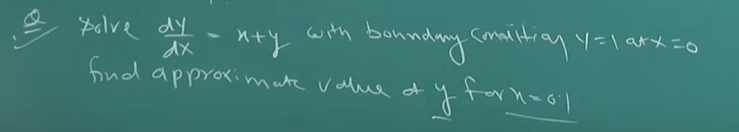
Note that this is NOT an explicit equation, but rather an ODE, so we don't need to find out the derivative ourselves.

In this case, the formula becomes :

Since our given $f(x,y)$ is already the derivative itself.

So we are given a starting condition as :

$y=1$ and $x=0$ and we need to find $y$ at $x=0.1$

Let's compute till $n=5$.

So the step size will be :

So using that we construct our table:

I got the values early on since I made a program to calculate all this

0, 0, 1, 1
1, 0.02, 1.0204, 1.0404
2, 0.04, 1.0416079999999999, 1.081608
3, 0.06, 1.0636401599999998, 1.1236401599999999
4, 0.08, 1.0865129632, 1.1665129632
5, 0.1, 1.110243222464, 1.210243222464
The value of y at x = 0.1 is: 1.110243222464 

However I will do some of them by hand to clear up any confusion.

So for $n=0$

Similarly for $n=1$

And so on... I assume you can do the rest of the calculations by yourself.

So the final approximation of $y(0.1)$ is $1.1102$.
And the value in the video was obtained as $1.108$ is due to precision differences.

2. Runge-Kutta Method (or Euler's Modified Method)

This method is used for 2nd order differential equations.

This is based upon Euler's method by modifying it.

(obtained by using Euler's method)

then, we use this to get :

Example 1:

Let's say we have :

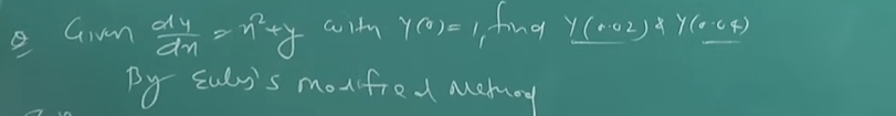
Another ODE, not an explicit equation.

We are given the starting conditions as $y(0)=1$ which means :

$x_0=0;y_0=1$

And we are asked to find the value of $y$ at $x=0.02$ and $x=0.04$

So if we continue till $n=5$, then the step size, $h$ will can be taken for simplicity purposes as :

$h=0.02$

Since we will be finding for two $x$ values and the difference between then is $0.02$ so for simplicity purposes we can take $0.02$

Or for better accuracy we can :

Let's find out which step size leads to more precise answer :

So, at $n=0andh=0.02$

We will have our table as :

We see that we can get the required $x_n$ values at a lesser number of iterations if we use $h=0.004$

And $$y_{1} \ = \ 1 \ + \frac{0.02}{2} \ \times [\ (0^2 \ + \ 1) \ + \ (0.02^2 \ + \ 1.02) ]$$

Now at $n=1$

Now,

So we have our as $y(0.02)=1.020204$ and $y(0.04)=1.030830282$