Index

1. Pre-requisites before heading into Linear Programming
2. Topic 1 Introduction to Optimization
3. Topic 2 Mathematical Formulation of Linear Programming Problems.
4. Topic 3 Feasible Solutions and the Feasible Region
5. Topic 4 Graphical Method of Solving Linear Programming Problems
6. Example 1 and Example 2
7. Basic Solution and Basic Feasible Solution
8. Degenerate Solution (or Degenerate-Basic Solution) and Non-Degenerate Solution (or Non-Degenerate-Basic Solution)
9. Convex Sets
10. The Simplex Method of solving Linear Programming Problems
11. The Algorithm of Simplex Method
12. Charnes' Big-M Method
13. Duality Theory

Pre-requisites before heading into Linear Programming

Topic 1: Introduction to Optimization

Before diving into Linear Programming, let's understand the fundamental concept of optimization.​

What is Optimization?

Optimization is the systematic process of finding the best possible solution to a problem from a set of available alternatives. In mathematical terms, it means finding values that either maximize or minimize a particular function while respecting certain limitations.​

Think of optimization problems everywhere in real life: a company wants to maximize profit while staying within budget constraints, a delivery service wants to minimize travel time while visiting all customers, or a factory wants to minimize production costs while meeting demand.​

Key Elements of Any Optimization Problem

Every optimization problem has three essential components :​

Decision Variables: These are the quantities you can control or modify to find the best solution. For example, if a bakery produces cakes and cookies, the number of cakes (let's call it $x_1$) and number of cookies ($x_2$) are decision variables.​

Objective Function: This is the mathematical expression you want to maximize or minimize. For the bakery, if each cake gives $10 profit and each cookie gives $5 profit, the objective function would be: Maximize Profit = $10x_1+5x_2$.​

Constraints: These are the restrictions or limitations that must be satisfied. The bakery has limited flour, sugar, oven time, etc. These limitations become constraints in mathematical form.​

What Makes It "Linear Programming"?

This brings us to a special type of optimization called Linear Programming (LP). Linear Programming is a method used when both the objective function AND all constraints can be expressed as linear equations or inequalities.​

The word "linear" here is crucial and connects directly to our (if you studied the whole section of Mathematics - 1A and Numerical Methods), linear algebra knowledge. In linear programming, all relationships between variables are linear—meaning variables appear with power 1 only, and terms are added or subtracted (no multiplication of variables with each other, no squares, no fractions with variables in denominators).​

The word "programming" here doesn't mean computer programming; it's an older mathematical term meaning "planning" or "scheduling".

Topic 2: Mathematical Formulation of Linear Programming Problems.

Now that we understand the three key components (decision variables, objective function, constraints), let's see how to write them mathematically and understand the different forms they can take.

General form of an LPP

A Linear Programming Problem in its general form looks like this:

Optimize(Maximize or minimize):

Subject to:

$a_{11}{x}_1+a_{12}{x}_2+\cdots +a_{1n}{x}_n\le \text{or}\ge \text{or}=b_1$

$a_{21}{x}_1+a_{22}{x}_2+\cdots +a_{2n}{x}_n\le \text{or}\ge \text{or}=b_2$

$⋮$

$a_{m1}{x}_1+a_{m2}{x}_2+\cdots +a_{mn}{x}_n\le \text{or}\ge \text{or}=b_m$

where $x_1,x_2,\cdots ,x_n$ are decision variables, $c_1,c_2,\cdots ,c_n$ are coefficients in the objective function, $a_{ij}$ are coefficients in constraints and $b_i$ are the the right-hand side constants.

Components Breakdown

Now let's understand what the components above actually mean:

Objective Function: The function $Z=c_1{x}_1+c_2{x}_2+\cdots +c_n{x}_n$ is what you're trying to optimize. The coefficients $c_1,c_2,\cdots c_n$
represent the contribution of each decision variable to your goal (like profit per unit, cost per item, etc.).

Constraints: These are the linear inequalities or equations that limit your choices. They can be of three types: $\le$ (less than or equal to), $\ge$ (greater than or equal to), or $=$ (equality).

Non-negativity Constraints: In most real-world problems, decision variables cannot be negative. You can't produce $-5$ chairs or invest -$100. This is why $x_i\ge 0$ for all decision variables.

Standard Form vs Canonical Form

For solving LPPs using algorithms (like the Simplex Method we'll learn later), we need to convert problems into specific standardized formats.

Canonical Form requires :​

• Objective function must be of maximization type
• All constraints (except non-negativity) must be ≤ type
• All variables must be non-negative
• Right-hand side values must be non-negative

Standard Form requires :​

• All constraints must be equalities (equations, not inequalities)
• This is achieved by introducing slack variables for $\le$ constraints and surplus variables for $\ge$ constraints​
• All variables (including slack/surplus) must be non-negative

Slack and Surplus Variables

To convert inequalities to equalities, we introduce new variables :

Slack Variable: Added to a $\le$ constraint. For example $2x_1+3x_2\le 10$ becomes $2x_1+3x_2+s_1=10$, where $s_1\ge 0$ . The slack variable represents the "unused" resource.

Surplus Variable: Subtracted from a $\ge$ constraint. For example, $4x_1+x_2\ge 8$ becomes $4x_1+x_2-s_2=8$ where $s_2\ge 0$. The surplus variable represents the "excess" over the minimum requirement.

Topic 3: Feasible Solutions and the Feasible Region

Types of Solutions

Feasible Solution: Any set of values for decision variables $(x_1,x_2,\cdots ,x_n)$ that satisfies all constraints (including non-negativity) is called a feasible solution. Think of it as any point that "plays by all the rules".

Infeasible Solution: Any solution that violates at least one constraint. These solutions are not acceptable.

Feasible Region (or Feasible Set): The collection of all feasible solutions forms a region in n-dimensional space. For two-variable problems, this is a region on the 2D plane.

For example in this diagram here:

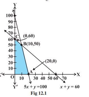
The shaded region OABC is the feasible region.

Optimal Solution: Among all feasible solutions, the one that gives the best (maximum or minimum) value of the objective function is called the optimal solution. An LPP can have a unique optimal solution, multiple optimal solutions, or no optimal solution (unbounded or infeasible cases).

Topic 4: Graphical Method of Solving Linear Programming Problems

https://www.youtube.com/watch?v=Bzzqx1F23a8 (must watch)

Step-by-Step Procedure: Corner Point Method

Step 1: Graph all constraints

Plot each constraint as a line on the xy-plane. For an inequality like $ax+by\le c$, first plot the line $ax+by=c$, then determine which side of the line satisfies the inequality(test the point.)

Step 2: Identify the feasible region

The feasible region is the area where all constraints overlap, including the non-negativity constraints $x\ge 0$, $y\ge 0$. This region lies in the first quadrant only. The feasible region will always be a convex polygon (or unbounded convex region)

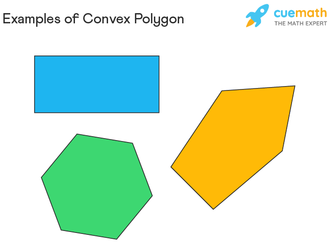
Here's few example images of a convex polygon:

Rules for finding the feasible region (very important)

• If both the constraints have $\le$ sign, then the feasible region will be to the left and below of the both the constraints, in the region where both of them overlap.

For example, this:

• If both the constraints have $\ge$ sign, then the feasible region will be to the right and above of both the constraints, making an unbounded region.

For example this:

• If the signs of the constraints are mixed, i.e. one constraint having a $\le$ sign and the other having a $\ge$ sign of vice-versa we would need to follow the appropriate rules for both the constraints to find the feasible region somewhere between the two constraints.

For example this:

Step 3: Find the corner points (vertices)

Corner points are where two constraint lines intersect. You can find them by solving pairs of equations simultaneously.

Step 4: Evaluate the objective function at each corner point

Calculate the objective function (for example if it is $Z=cx+dy$) at each corner point.

Step 5: Determine optimal solution

• Bounded region: The maximum (or minimum) value from Step 4 is your optimal solution.

• Unbounded region: If the region extends infinitely, you need to verify whether a maximum/minimum exists by checking if the half-plane $Z>M$ (for maximum) or $Z<m$ (for minimum) has common points with the feasible region.

Key Theorems

Theorem 1: If an optimal solution exists, it must occur at a corner point of the feasible region.

Theorem 2: If the feasible region is bounded, then both maximum and minimum values exist and occur at corner points.

Important: If two corner points give the same optimal value, then every point on the line segment joining them is also optimal (multiple optimal solutions).

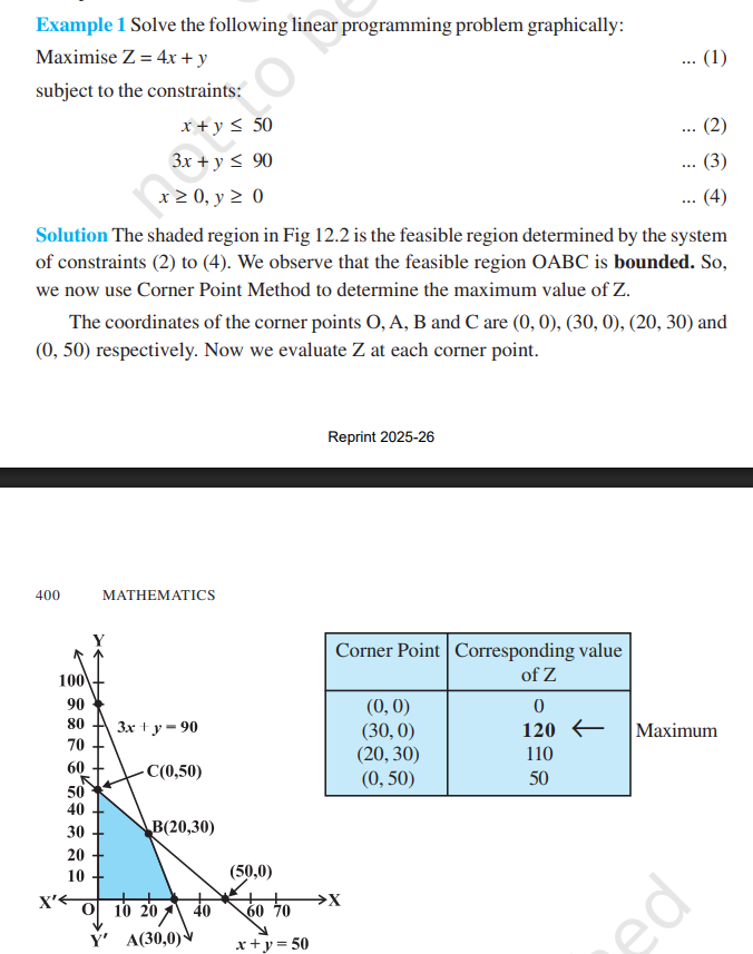
Example 1

Problem: Maximize $Z=4x+y$

Subject to:

• $x+y\le 50$
• $3x+y\le 90$
• $x\ge 0$, $y\ge 0$

Solution:

Step 1: Graph the constraints:

• Line 1: $x+y=50$.

In order to graph this line we will set both $x$ and $y$ to zero respectively to get:

$x=(50,0)$ and $y=(0,50)$.

• Line 2: $3x+y=90$

Setting $y=0$ , we get: $3x=90$, or $x=(30,0)$.

And setting $x=0$, we get: $y=90$, thus $y=(90,0)$.

• Line 3: $x\ge 0$, $y\ge 0$ is just the origin point.

Step 2: Find the feasible region

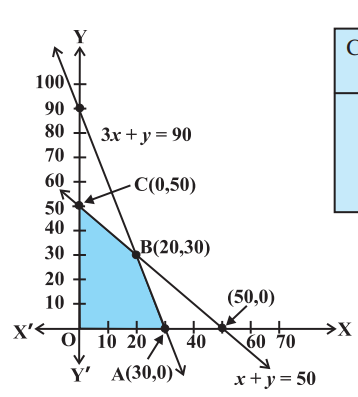
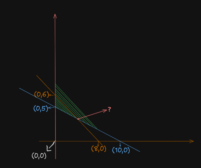
So, after plotting these lines, we find the feasible region as the region under which all the constraint lines overlap. In this case this one will be a neat bounded region:

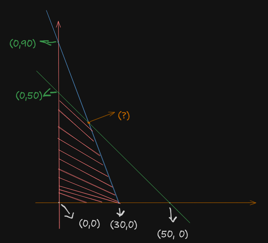
Assuming:

• $(0,0)$ as point $\text{O}$
• $(30,0)$ as point $\text{A}$
• The orange intersection point as $B$, which we have to calculate.
• $(0,50)$ as point $\text{C}$

The feasible region is $\text{OABC}$.

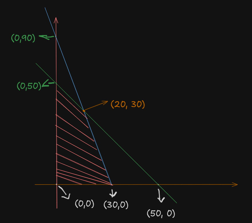
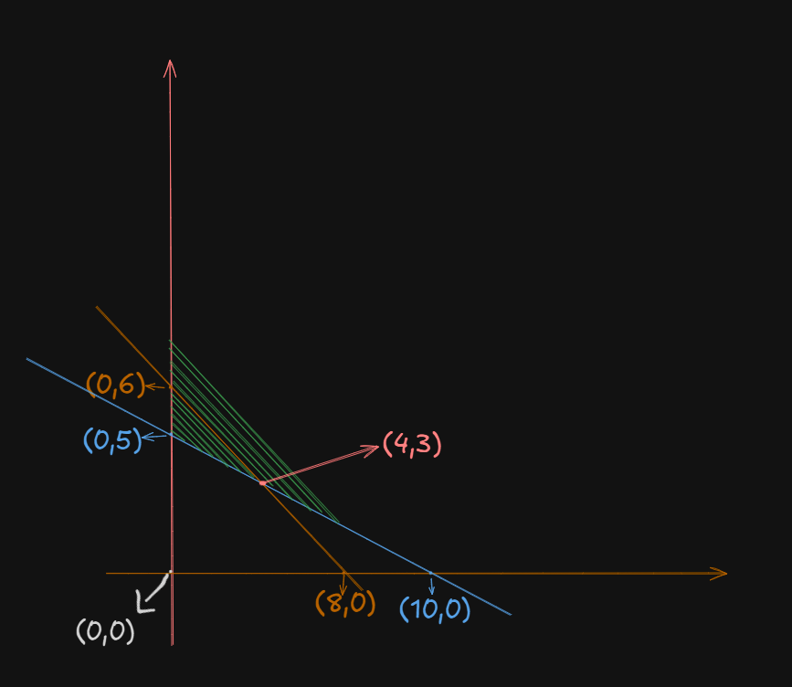
Step 3: Find all corner points

The only left to find is point B.

We can find out the intersection point by solving the two inequalities equations and getting their $x$ and $y$ values.

So we have:

• $x+y=50$
• $3x+y=90$

(Ignoring the $x\ge 0$, $y\ge 0$) since that won't get us any values and is just the origin.

A simple substitution would suffice here.

From $x+y=50$:

If we set: $x=50-y$

From: $3x+y=90$, substituting the value of $x$,

$⟹3(50-y)+y=90$

$⟹150-3y+y=90$

$⟹150-2y=90$

$⟹-2y=-160⟹y=30$

Now substituting the value of $y$ back in the first equation:

$x=50-30⟹x=20$

So we have:

• $(20,30)$ as point $\text{B}$

So, all our corner points are:

Step 4: Evaluate the objective function at corner points

So we evaluate $Z=4x+y$ at the corner points:

At origin $(0,0)$ , $Z=0$
At point A $(30,0)$, $Z=120$.
At point B $(20,30)$ , $Z=80+30⟹Z=110$.
At point C $(0,50)$, $Z=50$.

So,

Step 5: Find the maximum value from all the evaluated values of the objective function.

The maximum value is 120 at point (30, 0).

This means: produce 30 units of $x$ and 0 units of $y$ to maximize profit.

Here's the full reference of the example used:

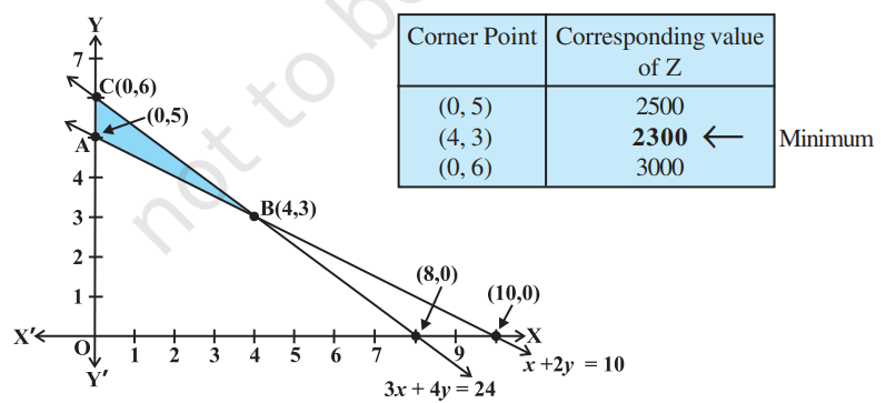
Example 2

Given objective function:

Subject to constraints:

• $x+2y\ge 10$
• $3x+4y\ge 24$
• $x\ge 0$, $y\ge 0$

For the first constraint, setting $x=0$

$2y=10⟹y=5$

And for $y=0$ : $x=10$

For the second constraint, setting $x=0$

$4y=24⟹y=6$

And for $y=0$: $x=8$

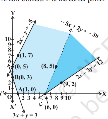
Now, we need to plot the feasible region. This one will be an unbounded region since both the constraints have the $\ge$ operator.

So, we get this:

Now, we have to find that intersection point.

• $x+2y\ge 10$
• $3x+4y\ge 24$

A simple substitution operation will suffice here:

Setting $x=10-2y$

In the second constraint:

$30-6y+4y=24$

$⟹30-2y=24$

$⟹-2y=-6$

$⟹y=3$

Applying $y=3$ back in the first constraint:

$x=10-6=4$

So, we get the intersection point at $(4,3)$

Now, to find the minimum, we evaluate $Z=200x+500y$ to at the existing corner points for the feasible region to find out the intersection point.

At point $(0,6)$: $Z=3000$
At point $(0,5)$: $Z=2500$
At point $(4,3)$: $Z=800+1500=2300$ which seems to the be the smallest out of all the values here.

So, the smallest value is $2300$ at $(4,3)$.

Basic Solution and Basic Feasible Solution

Converting to Standard form -- The how and the why.

Standard form is needed because the Simplex Method (an algebraic method we'll learn later) requires all constraints to be equations, not inequalities. The graphical method works fine with inequalities, but algebraic methods need equations.

Think of it like this: In linear algebra, when you solve systems of equations like $Ax=b$, you need equations, not inequalities.

A simple example

Problem: Maximize $Z=4x_1+x_2$

Subject to:

• $x_1+x_2\le 50$
• $3x_1+x_2\le 90$

Since it has a $\le$ operator, we add slack variables to convert ≤ to =

So, in standard form, the constraints are:

• $x_1+x_2+s_1=50$
• $3x_1+x_2+s_2=90$

where $s_1$, $s_2\ge 0$ are slack variables.

What are slack variables? They represent the "unused" amount of a resource. If the constraint is "at most 50," and you use 30, then the slack is 20.

Counting Variables: The Key to Everything

Now we count:

• Number of equations ($m$) : 2 (we have 2 constraints)
• Number of variables ($n$): 4 ($x_1$, $x_2$, $s_1$, $s_2$)

From linear algebra: A system with more variables than equations $(n>m)$ has infinitely many solutions.

Basic vs Non-Basic Variables: The simple rule

In a system with $m$ equations and $n$ variables:

• Choose $m$ variables to solve for: these are basic variables.
• Set the remaining $n-m$ variables to zero: these are non-basic variables.

From our example:

$m=2$ (we have two constraints)
$n=4$ (four variables)

So, $n-m=2$

That gives us:

• 2 basic variables
• 2 non-basic variables

Why do this?

Because when you have more variables than equations, you need to "fix" some variables to find a specific solution. By setting $n-m$ variables to zero, we reduce the problem to $m$ equations with $m$ unknowns, making the problem easier to solve using linear algebra.

Now let's solidify our understanding by finding one basic solution.

So we had:

• $x_1+x_2+s_1=50$
• $3x_1+x_2+s_2=90$

So, if we choose let's say $s_1$ and $s_2$ as the basic variables.

Then the remaining two variables $x_1$ and $x_2$ are the non-basic variables, which will be set to zero.

So, the constraints now become:

• $0+0+s_1=50$
• $0+0+s_2=90$

Thus the basic solution (the solution to the constraints) is:

$s_1=50$ and $s_2=90$

Since all values are $\ge$ 0, it's also a basic feasible solution.

Difference from regular feasible solutions

Regular feasible solution: ANY solution that satisfies all constraints. For example:

• $x_1=10$, $x_2=20$, satisfies both constraints
• $x_1=5$, $x_2=15$ also works

So there are infinitely many solutions.

whereas,

Basic feasible solution: A special feasible solution where exactly $n-m$ variables are zero. For example:

• $x_1=0$, $x_2=0$ (we already did this just now)
• $x_1=30$, $x_2=0$
• And so on, but only a finite number of basic feasible solutions exist.

The Key Insight

Basic feasible solutions are the corner points we've been graphing! At each corner point.

• Exactly 2 variables are non-zero (basic)
• Exactly 2 variables are zero (non-basic)

This is why we only check corner points in the graphical method.​

Now, as to part of "where do the basic variables need to be selected from, can it be from one constraint, or both?"

You can choose basic variables from anywhere (same constraint, different constraints, doesn't matter) as long as their corresponding columns in the constraint matrix are linearly independent. We learnt about linear independence back in Module 3 -- Matrices#Linear Independence

However, if you are worried about the time it would take to test the combination of variables:

In practice:

• Slack variables often form a natural basis because they give an identity matrix (best for basic variables)​

• The Simplex Method algorithmically ensures the chosen basis is always valid​.

• You don't manually check every combination - algorithms do this for you.

Degenerate Solution (or Degenerate-Basic Solution) and Non-Degenerate Solution (or Non-Degenerate-Basic Solution)

A basic feasible solution (BFS) is called:

Non-Degenerate BFS: When all basic variables are strictly positive (greater than zero).

Degenerate BFS: When at least one basic variable equals zero.

That's basically it.

Why Does This Matter?

Degeneracy can cause problems in the Simplex Method :​

• It may lead to cycling (going in circles without reaching the optimal solution)​.
• It requires extra iterations without improvement in the objective function​.
• Multiple bases can lead to the same solution.

Concrete Example: Non-Degenerate Basic Feasible Solution

Using our maximizing problem again:

• $x_1+x_2+s_1=50$
• $3x_1+x_2+s_2=90$

BFS at corner point (20, 30):

• Basic variables: $x_1=20$, $x_2=30$
• Non-basic variables: $s_1=0$, $s_2=0$

Is this degenerate? NO! Both basic variables ($x_1$ and $x_2$) are positive (20 and 30). This is a non-degenerate BFS.

Concrete Example: Degenerate Basic Feasible Solution

Let's consider a different problem:

We have 3 constraints:

• $x_1+x_2+s_1=10$
• $2x_1+s_2=0$
• $x_1+3x_2+s_3=15$

We have 3 constraints: $m=3$. We have 3 basic variables.
We have 5 variables: $n=5$

To find basic variables we need to set $n-m$ or $5-3=2$ variables to zero.

Now, suppose we get this basic feasible solution:

• Basic variables: $x_1=0$, $x_2=5$, $s_3=0$
• Non-basic variables: $s_1=5$, $s_2=0$

Is this degenerate? YES! One of the basic variables ($x_1=0$) equals zero. This is a degenerate BFS.

Geometric Interpretation

Non-degenerate corner point: Exactly $m$ constraints are "tight" (active) at that point, where $m$ is the number of equations.​

In 2D with 2 constraints: A non-degenerate corner point is where exactly 2 constraint lines intersect.​

Degenerate corner point: More than $m$ constraints pass through the same point.​

In 2D: If 3 or more constraint lines meet at the same point, that corner point is degenerate.

Convex Sets

A set is convex if, when you pick any two points inside it, the entire line segment connecting those two points also lies completely inside the set.

Think of it as: "no dents, no holes, no curves inward".

In simple words, we can explain the convex set as a shape. Imagine a shape or a group of points. A set is called convex if, whenever you pick any two points inside it, the straight line connecting those two points also stays completely inside the shape.

For example take these shapes:

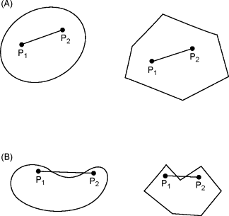
In section (A), in both shapes, the line connecting points $P_1$ and $P_2$ is completely within the shape, as opposed to section (B) where the line can be seen going out of the shapes' boundary by a bit.

The shapes in section A are convex sets, while those in section B are not.

Simple Examples

Convex Sets:

• Circle: Pick any two points inside a circle, the line between them stays inside
• Square: Any line segment between two points in a square stays in the square
• Triangle: Always convex
• Any polygon without indentations (regular shapes)
• Half-space: The region defined by $ax+by\le c$
• Your feasible regions from the graphical method problems!

Non-Convex Sets:

• Crescent moon: If you pick two points on opposite ends, the line between them goes outside
• Star shape: Lines between points on opposite arms go outside
• Letter "C": Connect the top and bottom of the C - the line segment is outside
• Donut/Ring: Any line through the hole exits the set

Why Feasible Regions Are Always Convex

This is a fundamental theorem in linear programming :​

The feasible region of a linear programming problem is ALWAYS convex.​

Why? Each constraint creates a half-space (a convex set), and the intersection of convex sets is always convex.

The Simplex Method of solving Linear Programming Problems

What is the Simplex Method?

The Simplex Method is an iterative algebraic algorithm that solves linear programming problems by systematically moving from one corner point (basic feasible solution) to another, always improving the objective function, until the optimal solution is reached.​

Think of it as: Instead of graphing and checking all corners visually, the Simplex Method does this algebraically using a table (called a tableau)

Why Do We Need It?

The graphical method only works for 2 or 3 variables. For real-world problems with hundreds or thousands of variables, we need an algebraic approach. The Simplex Method can handle any number of variables.

The Algorithm of Simplex Method

Step 1: Convert to Standard Form

• Maximize (if minimizing, convert by multiplying objective by -1)
• All constraints must be equalities (add slack variables)
• All variables $\ge 0$
• All RHS values $\ge 0$

Step 2: Create the Initial Simplex Tableau

• Write the problem as a table with rows for constraints and one row for the objective function.

• Include all variables (original + slack)

Step 3: Identify the entering variable (pivot column)

• Find the most negative entry in the objective row (bottom row).

• The column with this entry becomes the pivot column.

• This variable will enter the basis (become basic).

Step 4: Identify the Leaving Variable (Pivot Row)

• Calculate minimum ratio test: Divide the elements of RHS by it's corresponding pivot column entry (dividing only positive entries from the RHS, excluding the RHS element from the objective function row).

• The row with the smallest ratio becomes the pivot row (Ignore negative and zero values).

• This variable will leave the basis (become non-basic)

With having both the pivot row and column pinned down, we can identify the pivot element itself.

Step 5: Perform Pivot Operation

• Make the pivot element = 1 (divide pivot row by pivot column)

• Make all other entries in pivot column zero (basically follow Gaussian Elimination)

Step 6: Check for optimality

• If all entries in the objective row are $\ge 0$, that's the time to stop the algorithm.

• If there are still negative entries, loop back to step 3.

Step 7: Read the Solution

• Basic variables (columns with single 1 and rest 0s) have values from RHS

• Non-basic variables = 0

• Objective function value is in the RHS of the objective row

Example

Let's understand the method by going though with a simple yet concrete example.

Let's solve this problem step by step:

Maximize $Z=3x_1+2x_2$

Subject to:

• $2x_1+x_2\le 18$
• $2x_1+3x_2\le 42$
• $3x_1+x_2\le 24$
• $x_1,x_2\ge 0$

Step 1: Convert to standard form.

We do this by adding slack variables.

• $2x_1+x_2+s_1=18$
• $2x_1+3x_2+s_2=42$
• $3x_1+x_2+s_3+24$

Objective: $Z-3x_1-2x_2=0$

Step 2: Initial Simplex Tableau

The initial variables in the basis are the 3 basic variables, chosen as $s_1$, $s_2$ and $s_3$ along with the result of the objective function, $Z$, since slack variables by default are the most suitable basic variables.

Step 3: Identify the entering variable for the basis.

Iteration 1.

First, a quick re-write of the table as a proper matrix:

The most negative variable in the row of the objective function is $x_1=-3$

This way, we identified the pivot column in the matrix, which will be used later for row operations via Gaussian Eliminations

Step 4: Identify the leaving variable for the basis.

Minimum ratio test:

• Row 1: $\frac{18}{2}=9$
• Row 2: $\frac{42}{2}=21$
• Row 3: $\frac{24}{3}=8\leftarrow \text{minimum}$.

Minimum is $8$, so $s_3$ leaves.

Step 5: Pivot Operations.

So we have our matrix:

I added the column names back to keep track of which is our pivot column (the one in which our entering variable is in.)

Our pivot: $R_{31}=3$.

Goal 1: Convert all elements in Objective row (the last row) to either zero or greater than zero.

Applying row operations:

$R_4\to R_4+R_3$

There is still one negative value remaining, the $x_2=-1$

However before that, to make things simpler, let's reduce the pivot to 1.

$R_3\to \frac{R_3}{3}$.

We can better format the fractional values to decimal:

Before we proceed to fully eliminate the -1, we have to reduce all the other elements in the current pivot column to zero.

So,

$R_2\to R_2-2R_3$

Now, for $R_1$,

$R_1\to R_1-2R_3$

That concludes iteration 1.

Iteration 2

Now, we are ready to work on the objective row again.

Most negative element in objective row is $-1$, under $x_2$.

So $x_2$ enters the basis.

Now, to find the leaving variable:

• Row 1: $\frac{2}{0.34}=5.88\to \text{minimum}$
• Row 2: $\frac{26}{2.34}=11.11$
• Row 3: $\frac{8}{0.33}=24.24$

Minimum is $5.88$, so $s_1$ leaves.

Now we have our new pivot sitting at row 1, column 2, which is $0.34$.

First we normalize the pivot to 1:

$R_1\to \frac{R1}{0.34}$

So, for $R_4$:

$R_4\to R_4+R_1$

Now we still have a negative value under $s_3$, so, that leads to one more iteration.

Before we proceed to iteration 3, we need to reduce all the other non-pivot elements in the pivot row to zero.

For $R_2$:

$R_2\to R_2-2.34\times R_1$

For $R_3$:

$R_3\to R_3-0.33\times R_1$

This marks the end of iteration 2.

Iteration 3

Now we repeat the same process again.

Most negative element is under $s_3$ which is -0.94

That's our pivot column. $s_3$ enters the basis

Now we test the minimum ratios:

• Row 1: $\frac{5.88}{-1.94}=-3.03$ (ignoring)
• Row 2: $\frac{12.24}{3.87}=3.16\to \text{minimum}$
• Row 3: $\frac{6.05}{0.97}=6.23$

$s_2$ leaves the basis.

So, we have our pivot on $R_{25}$.

First we normalize the pivot.

$R_2\to \frac{R_2}{3.87}$

Now, for $R_4$ :

$R_4\to R_4+0.94\times R_2$

Now, we just need to convert the remaining non-pivot elements to zero.

Starting with $R_{15}$.

$R_1\to R_1+1.94\times R_2$

And for $R_{35}$:

$R_3\to R_3-0.97\times R_2$

Since no elements on the objective function row are less than zero, we have reached optimality and now, can stop.

Step 6: Reading the solution

We identify columns that have:

• Exactly one 1
• All other entries are 0

The candidates are:

$x_1$, $x_2$ and $s_3$.

So these are our basic variables.

We construct a proper matrix:

So,

• $x_2=12.01$
• $s_3=3.16$
• $x_1=2.99$

That's our basic feasible solution.

Charnes' Big-M Method

Big-M Method : The Core Idea

The Big-M Method solves a fundamental problem: What if you can't use slack variables to get an initial basic feasible solution?

The Problem

In our previous problem, all constraints were of type: $\le$

For example:

• $x_1+x_2\le 50$
• $3x_1+x_2\le 90$

We easily added slack variables to get our starting point (0,0).

But what if we have $\ge$ or $=$ constraints?

• $x_1+x_2\ge 10$
• $2x_1+3x_2=50$

Now, the problem is that we can't start at (0,0) - it violates these constraints!

The Big-M Solution: Artificial Variables

Idea: Add "artificial variables" to create a valid starting point, but make them so undesirable that they get kicked out immediately.

How? Assign them a huge penalty (M = very large number) in the objective function :

• Maximization: Add -M × (artificial variable) → makes it very bad​
• Minimization: Add +M × (artificial variable) → makes it very bad

When Do You Need Big-M?

​

The Big-M Algorithm (5 Steps)

Step 1: Make all RHS positive (multiply by -1 if needed)

Step 2: Convert constraints to equations:

• $\le$ constraint: Add slack variable $s_i$
• $\ge$ constraint: Subtract surplus variable $e_i$, add artificial $a_i$
• $\text{=}$ constraint: Add artificial variable $a_i$

Step 3: Modify objective function:

• Maximization: $Z^{\prime }=Z-M\sum a_i$
• Minimization: $Z^{\prime }=Z+M\sum a_i$

Step 4: Create initial tableau and eliminate artificial variables from Z-row.

Step 5: Solve using regular Simplex (we know this part).

Key Differences from Regular Simplex

Example

Let's cement the understanding using a concrete example

Given:

Maximize $Z=3x_1+2x_2$

Subject to:

• $x_1+x_2\ge 4$
• $2x_1+x_2\le 10$
• $x_1,x_2\ge 0$

Step 2: Convert constraints

• Constraint 1: $x_1+x_2-e_1+a_1=4$ (surplus + artificial)
• Constraint 2: $2x_1+x_2+s_1=10$ (that's our usual slack variable)

Step 3: Modified objective function

$Z=3x_1+2x_2-M{a}_1$

In standard form: $Z-3x_1-2x_2+M{a}_1=0$

Step 4: Initial Tableau (before elimination of artificial variables)

Let the initial chosen basic variables be: $a_1$ and $s_1$

Step 5: Eliminate artificial variable from Z-row.

We need to make the $a_1$ column have 0 in the Z-row.

So, we can go for this row operation:

$Z\to Z-M\times R_1$

Thus:

From here on out, we can apply the The Simplex Method of solving Linear Programming Problems and solve this problem to get the correct basic variables and their solution.

Since the method is way too much calculation intensive, I won't bother with the calculations this time.

However you may have some questions remaining:

QUESTION 1: Won't M in Z-row Affect Simplex Operations?

Answer: YES, and that's exactly the point!

The M terms in the Z-row are INTENTIONAL and guide the Simplex algorithm.

How M Works During Simplex

Remember: M is assumed to be infinitely large (M → ∞)

When comparing Z-row entries for the entering variable:

text

Z-row: -3-M -2-M M 0 0

Which is most negative?

Since M is huge:

• (-3-M) is MUCH more negative than (-2-M)
• Both are MUCH more negative than 0
• M is positive

Order: (-3-M) < (-2-M) < 0 < M

So $x_1$ with coefficient (-3-M) is the most negative, making it the entering variable.

The M Terms Stay Throughout

The M terms remain in the Z-row during iterations. They only disappear when:

1. Artificial variables leave the basis (get eliminated)
2. You reach the optimal solution

This is normal and expected!

QUESTION 2: Why is 0 in a1 Column Enough? There's Still a 1 Above!

Answer: The 1 is PERFECTLY FINE! That's how basic variables work.

Understanding Basic Variable Columns

Look at our final tableau after the removal of multiplier:

The a1 column is: (reading top to bottom including Z-row) is a unit column -- exactly what we need for a basic variable!

Why the 1 is Necessary

The 1 in the a1 column (Row 1) tells us:

• $a_1$ is in the basis
• $a_1=4$ (from RHS of Row 1)
• The constraint equation is satisfied

This is identical to regular Simplex!

The top 1 stays - it MUST stay to indicate a1 is basic!

With that, we can conclude the Big-M method.

Duality Theory

The Core Concept

Every LP problem (called the PRIMAL) has a paired problem (called the DUAL). They're like two sides of the same coin - solving one gives you information about the other!

The Primal-dual relationship

Example to understand the concept.

Primal problem:

Maximize $Z=50x_1+30x_2$

Subject to:

• $4x_1+3x_2\le 100$
• $3x_1+5x_2\le 150$
• $x_1,x_2\ge 0$

Now the dual variant of this problem would be:

Minimize $G=100y_1+150y_2$

Subject to:

• $4y_1+3y_2\ge 50$
• $3y_1+5y_2\ge 30$
• $y_1,y_2\ge 0$

How to construct the dual equation?

The Transformation Rules

Step 1: Flip the objective

• Primal MAX becomes Dual MIN
• Primal MIN becomes Dual MAX

Step 2: Transpose the coefficient matrix

• Primal rows become dual columns
• Primal columns become dual rows

Step 3: Swap coefficients and constraints

• Primal objective coefficients become dual RHS
• Primal RHS becomes dual objective coefficients

Step 4: Reverse inequalities

• Primal <= becomes dual >=
• Primal >= becomes dual <=
• Primal = stays dual =

Think of it as "Everything swaps roles"

Example

Given primal equation:

Maximize Z = 3x1 + 5x2

Subject to:

• x1 + 2x2 <= 6

• 2x1 + x2 <= 8

• x1, x2 >= 0

CONSTRUCT DUAL:

Step 1: Flip objective
Primal MAX → Dual MIN

Step 2: Create variables
2 constraints → 2 dual variables: y1, y2

Step 3: Dual objective
RHS values (6, 8) become coefficients
Dual: MIN G = 6y1 + 8y2

Step 4: Dual constraints
For x1 (column , objective coefficient 3):​
1y1 + 2y2 >= 3

For x2 (column , objective coefficient 5):​
2y1 + 1y2 >= 5

Step 5: Variable signs
Primal has <= → Dual variables >= 0
So: y1, y2 >= 0

FINAL DUAL:

Minimize G = 6y1 + 8y2

Subject to:

• y1 + 2y2 >= 3

• 2y1 + y2 >= 5

• y1, y2 >= 0