Module 2 -- Network Analysis -- Operations Research
Index
- 1. The Floyd-Warshall Algorithm
- 2. Ford-Fulkerson Algorithm
- The Maximal Flow(or sometimes known as "Maximum Flow") Problem
- The Backward Edge cases and why backward edges are helpful (important)
- Network Analysis PERT and CPM
- Important Terminologies for network diagrams
- Example 1 Drawing a basic network diagram.
- Critical Path Method (CPM)
- Finding the Critical Path.
- PERT (Program Evaluation and Recommendation Technique)
- Important terminologies
- Example
- Inventory Control Economic Order Quantity (EOQ)
Shortest Path Algorithms
1. The Floyd-Warshall Algorithm
Referenced from Fundamental Algorithmic Strategies, Graph and Tree algorithms#Floyd-Warshall Algorithm (from DAA)
The Floyd-Warshall algorithm is used to find the shortest paths between all pairs of vertices in a weighted graph. It's particularly useful for dense graphs and can handle both positive and negative edge weights, but not negative cycles.
Simple Explanation
Imagine you have a map of cities connected by roads, and you want to find the shortest path between every pair of cities. The Floyd-Warshall algorithm systematically updates the shortest paths by considering each city as an intermediate point and checks if passing through this city offers a shorter path between two other cities.
Steps of the Algorithm
-
Initialize the Distance Matrix: Create a matrix
distwheredist[i][j]represents the shortest distance from cityito cityj. Initially, setdist[i][j]to the weight of the edge betweeniandjif it exists; otherwise, set it to infinity. Setdist[i][i]to 0 for alli. -
Update the Distance Matrix: For each pair of cities
(i, j), consider each citykas an intermediate point. Updatedist[i][j]to be the minimum ofdist[i][j]anddist[i][k] + dist[k][j]. This means if passing throughkoffers a shorter path fromitoj, update the shortest path. -
Repeat for All Cities: Repeat the update step for all cities
k.
By the end of this process, dist[i][j] will contain the shortest distance from city i to city j.
Or in simple terms, observe the below stuff
Visual Aid
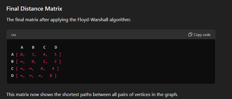
Imagine a graph with four cities (A, B, C, D) and the following distances between them:
- A to B: 3
- A to C: 10
- B to C: 1
- B to D: 2
- C to D: 4
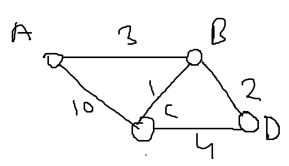
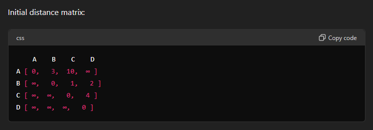
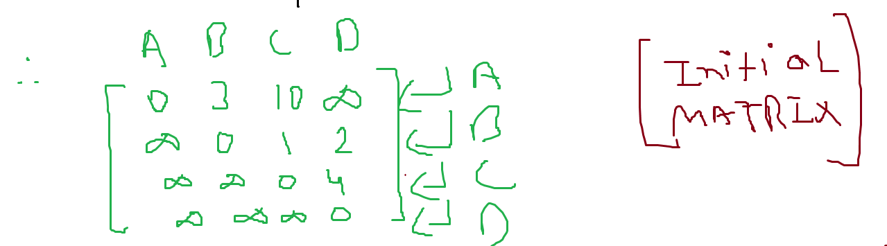
Here each row, each vertex is considered an intermediate point.
In this case, A sets the distance to itself as 0, and we write the rest of the distances from A to other vertices.
In the second row, B is set as the intermediate point. And we do the same for B. Note that from B's perspective the vertex before it is already considered and thus is set to infinity and not considered anymore.
In the third row, C is set as the intermediate point. And we repeat the same for C.
In the last row, D is set as the intermediate point. And we repeat the same for D.
Now we find from the graph that two shortest distances appear when we consider A as an intermediate point.
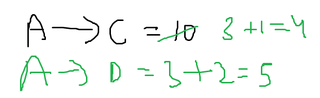
A to C is previously set as 4 and A to D is set as infinity but now :

In the updated distance matrix, we find shortest distances for the pair of cities C and D through A being an intermediate point.

Now this content was copied from my semester 4 notes, back when I was in a real hurry to get things done so that's why half of the content is in text and the other screenshots taken from ChatGPT.
However I hope this should suffice as a really good explanation of the algorithm.
2. Ford-Fulkerson Algorithm
https://www.youtube.com/watch?v=NwenwITjMys
Important Terminologies to know for the maximal flow problem using ford-fulkerson algorithm
-
Source: The node of the graph from which all the edges are in the outgoing direction. It is the starting/originating node of the graph.
-
Sink: The node of the graph to which all the edges from the other nodes are incoming. It is also the final node of the graph.
-
Capacity: The capacity of an edge is the maximum amount of value that particular edge can have.
-
Bottleneck capacity: The bottleneck capacity is measured in "paths", where a path can be the combination of multiple edges from the source to sink. The bottleneck capacity's value of that particular path is the minimum capacity out of all the edges involved in that path.
-
Flow: The flow, is measured edge wise, is the current value of the edge. It's written on the left side of the dividing line, the right side indicating the capacity of that particular edge.
-
Augmenting path: This is the path that is being taken from the source to the sink
-
Residual Capacity: Every edge has something called residual capacity. This is obtained by:
The Maximal Flow(or sometimes known as "Maximum Flow") Problem
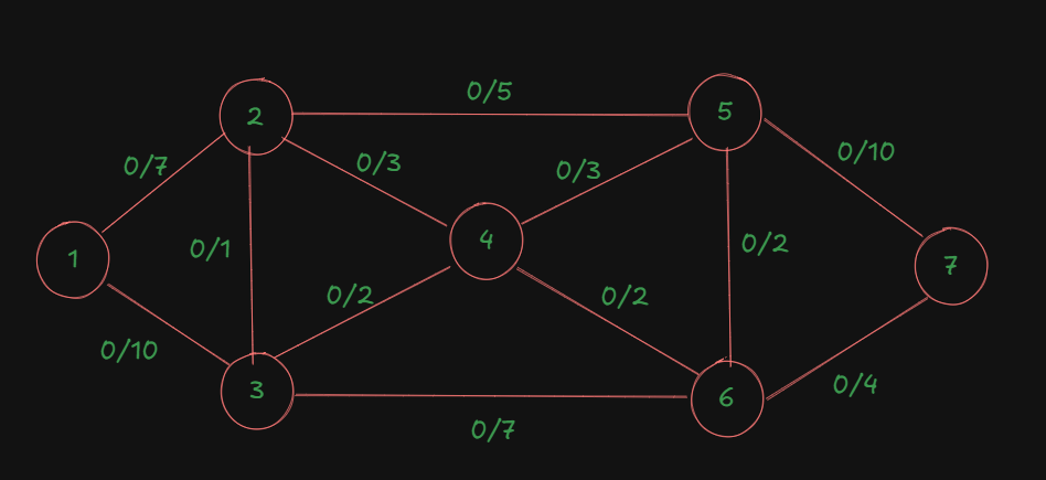
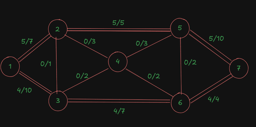
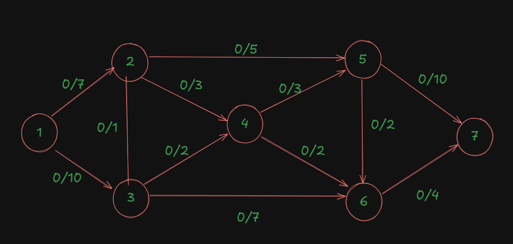
Let's understand this problem with the help of a graph.
As you can see, all the edges are marked up with the left side of the marking indicating their current flow, which is zero, and on the right, each edge's maximum capacity.
This table right here will be useful for getting the maximal flow out of the system since all we need to do is trace all the augmented paths from the source to the sink, find the bottleneck capacities per path, then add them to get the maximal flow.
| Augmented Path | Bottleneck Capacity/Flow for the path |
|---|---|
| 1-2-5-7 | |
For the first path:
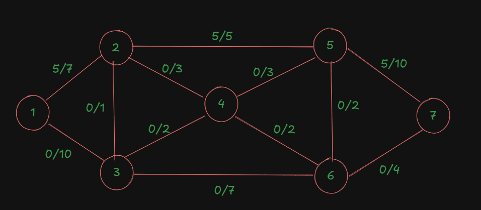
We have the bottleneck capacity as 5, since the it's the minimum out of the total capacities of all the edges in the path.
So, flow for the first path is 5.
Now the diagram is updated, with the last used path having double edges as an indication that that path cannot be reused again.
So, we update the table:
| Augmented Path | Bottleneck Capacity/Flow for the path |
|---|---|
| 1-2-5-7 | 5 |
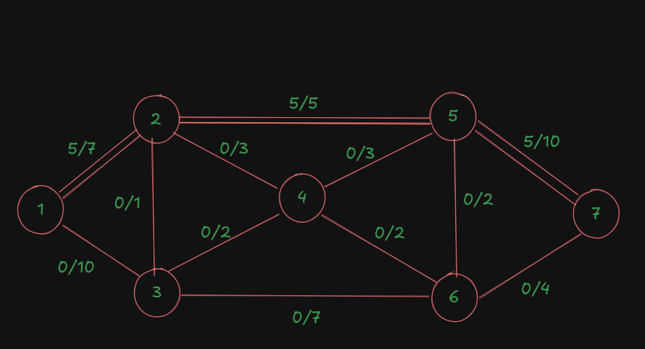
| 1-3-6-7 | |
For the second path:
The bottleneck capacity is: 4.
So, we update the table:
| Augmented Path | Bottleneck Capacity/Flow for the path |
|---|---|
| 1-2-5-7 | 5 |
| 1-3-6-7 | 4 |
| 1-2-4-5-7 | |
Now, for this path:
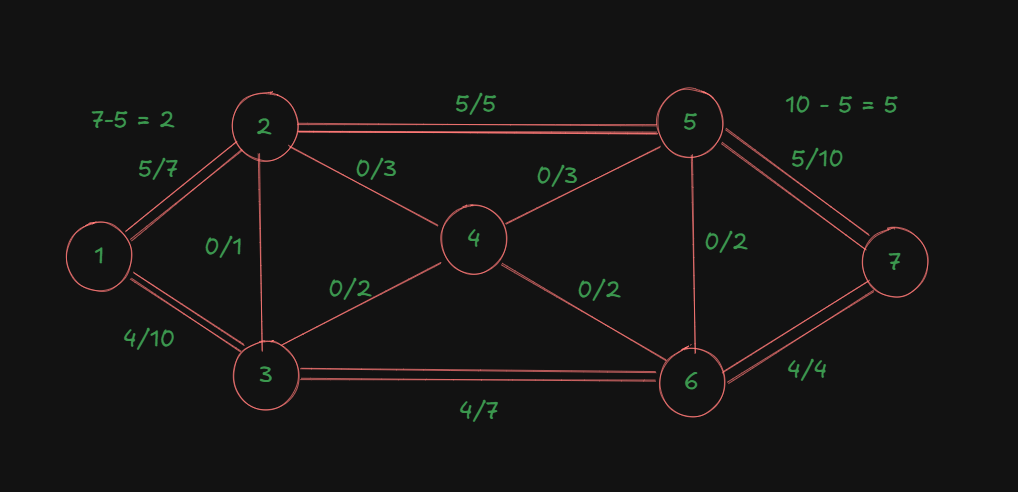
For the edge of node 1 to node 2, we already had an ongoing flow of 5, out of the max capacity of 7.
For the edge of node 5 to node 7, we already had an ongoing flow of 5, out of the max capacity of 10.
The other two edges currently have no ongoing flows.
So, to find the bottleneck capacity here, we need to consider the remaining capacities of all the edges involved in the path.
For the first edge, that would be
For the last edge, that would be
The other edges both have 3 as their remaining capacities.
The minimum out of all these capacities is 2.
So that's our bottleneck capacity for this path.
So we are adding an additional flow of 2 to all the involved edges in the path.
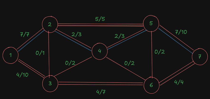
That's our updated diagram:
| Augmented Path | Bottleneck Capacity/Flow for the path |
|---|---|
| 1-2-5-7 | 5 |
| 1-3-6-7 | 4 |
| 1-2-4-5-7 | 2 |
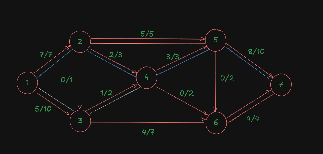
| 1-3-4-5-7 |
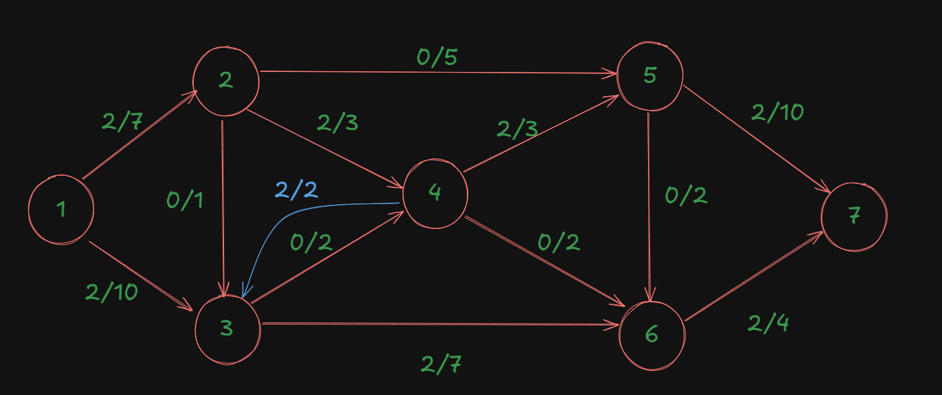
A slight update to our diagram, since in these type of problems we are always dealing with the directed graphs, apologies for the late update:
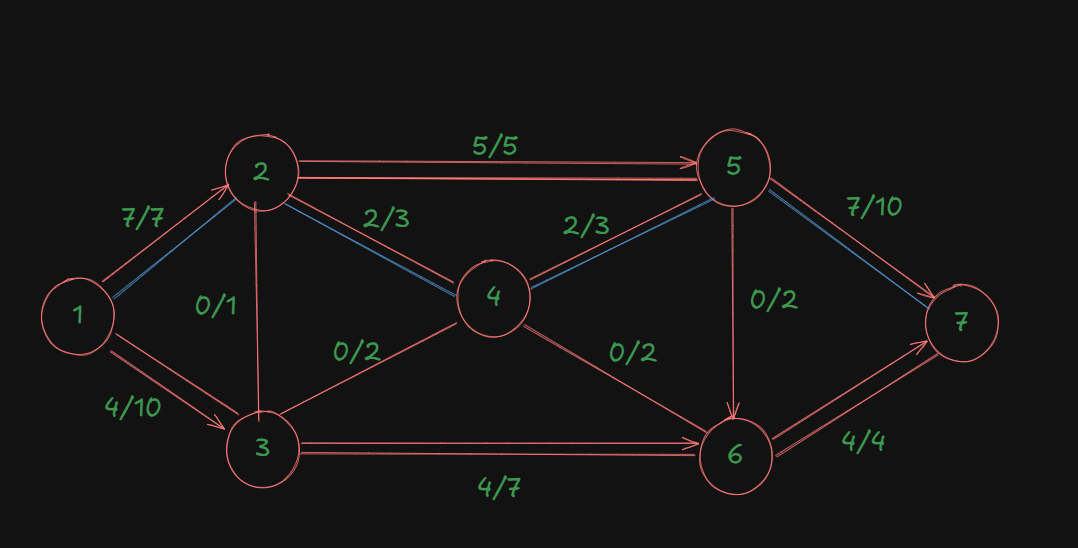
Now let's check for this path.
For nodes 1-3: residual capacity = 10-4 = 6
For nodes 3-4: residual capacity = 2-0 = 2
For nodes 4-5: residual capacity = 3-2 = 1
For nodes 5-7: residual capacity = 10-7 = 3
The minimum out of all these is 1.
That's the new bottleneck capacity.
| Augmented Path | Bottleneck Capacity/Flow for the path |
|---|---|
| 1-2-5-7 | 5 |
| 1-3-6-7 | 4 |
| 1-2-4-5-7 | 2 |
| 1-3-4-5-7 | 1 |
The updated diagram will be:
Let's check if there are any further available paths:
Edge 1-2 : blocked.
Edge 1-3: available.
Edge 3-4: available.
Edge 3-6: available.
Edge 6-7: blocked.
Edge 4-5: blocked.
Edge 4-6: available.
That leads us back to edge 6-7 which is blocked.
So, no further paths can be made. Since we have an edge 5-6 not 6-5, the path is available if we could get to node 5 anyhow but that's not possible.
So we end the process here and add up the flow values.
| Augmented Path | Bottleneck Capacity/Flow for the path |
|---|---|
| 1-2-5-7 | 5 |
| 1-3-6-7 | 4 |
| 1-2-4-5-7 | 2 |
| 1-3-4-5-7 | 1 |
| Maximal Flow | 12 |
Thus, the maximal flow in this system using ford-fulkerson algorithm is 12.
The Backward Edge cases and why backward edges are helpful (important)
So far, in our problem, we managed to get the maximal flow properly since the chosen paths were already the most optimal paths.
However, Ford-Fulkerson algorithm is a greedy algorithm, and it tends to get stuck in local optima. To prevent this from happening and correcting the flow when needed, we need backward edges.
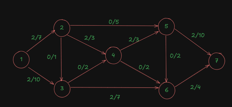
Let's go back to our original diagram again.
Assume the same directed edges:
1->2, 1->3, 2->3, 2->5, 2->4, 3->4, 3->6, 4->5, 4->6, 5->6, 5->7, 6->7
Let's say instead of our smart path choices, we make this greedy but suboptimal choice first:****
Instead of path 1->2->5->7 we choose 1 → 3 → 4 → 5 → 7.
Residual capacities:
- Edge 1->3: 10
- Edge 3->4: 2
- Edge 4->5: 3
- Edge 5->7: 10
Bottleneck capacity = 2 (limited by edge 3->4)
After pushing 2 units of flow, the graph becomes:
- Edge 1->3: 2/10
- Edge 3->4: 2/2 (saturated!)
- Edge 4->5: 2/3
- Edge 5->7: 2/10
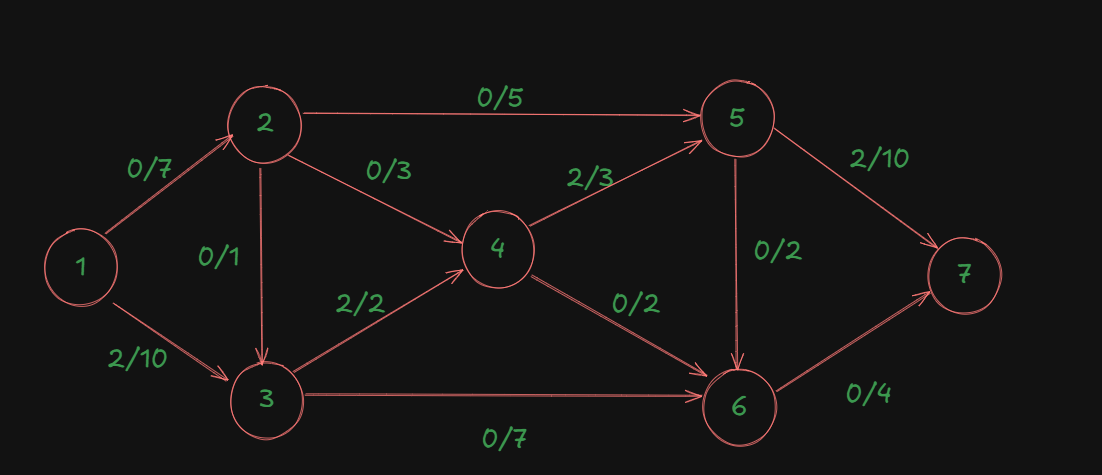
The Problem
Now you're stuck if you don't use backward edges! Edge 3->4 is completely saturated, but this blocks better paths. Without backward edges, you might only achieve a flow of 10 or 11, missing the optimal 12.
But what is this backward edge?? Is it something we create?
The answer is: No! The backward edge is automatically created by the algorithm, for the purposes of rerouting the flow so that an alternative optimal path may be found from the source to the sink, instead of jamming that particular edge and blocking all possible future optimal paths via that edge.
Here is the path construction rule involving backward edges.
For every edge
if current_flow > 0:
    Add backward edge (v->u) with capacity = current_flow

if (capacity - current_flow) > 0:
    Keep forward edge (u->v) with capacity = capacity - current_flow
So, in the residual graph, we will have a new edge:
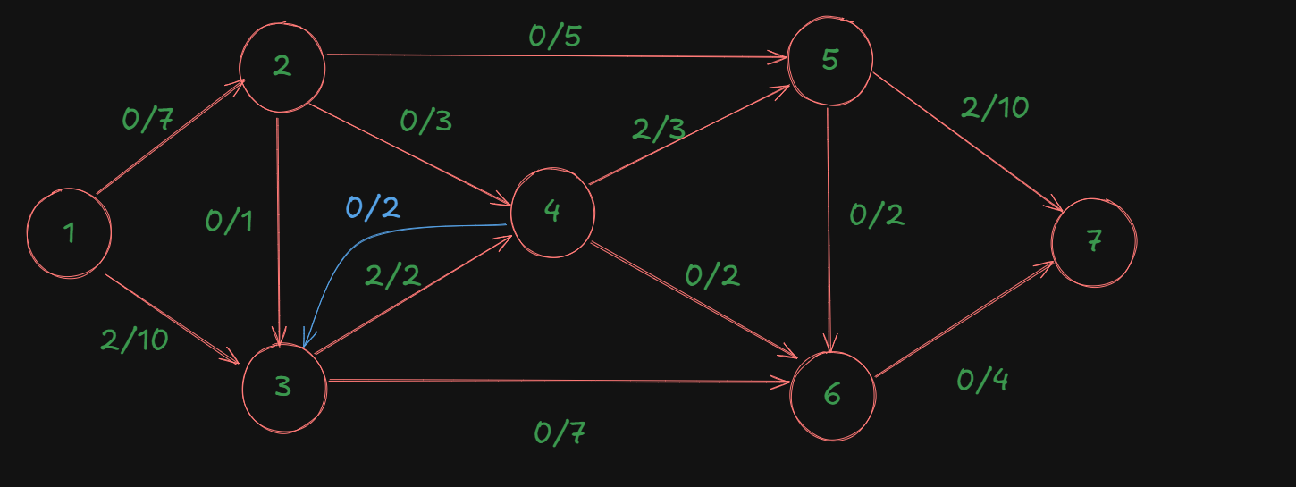
Now we can start finding a new augmenting path through the backward edge from source to sink.
For the path:
1->2->4->3->6->7
The capacities of each edge:
1->2: 7
2->4: 3
4->3: 2
3->6: 7
6->7: 4
The minimum out of this is: 2, which is also the flow for this path and one of the optimal flows we found earlier.
So the graph becomes:
As we can see, using this backward edge, the flow is literally rerouted from the node 4, thus unblocking the edge 3->4, and finding the better path.
After this, the backward edge will disappear, leaving our graph as:
So then what of the path we took using the backward edge?
Well that's the thing about backward edges, these are temporary, so the paths constructed using them also temporary, what matters are the final flow values we get from those paths.
What Really Matters
Focus on the edge flows, not the specific paths.
Key Points
-
Augmenting paths are temporary tools: They help you figure out how to update flows during each iteration, but once that iteration is done, the path itself doesn't matter anymore.
-
Edge flows are what persist: After each iteration, only the updated flow values on edges matter. These accumulate throughout the algorithm.
-
The final maximum flow value is all that counts: Ford-Fulkerson guarantees that when no more augmenting paths exist, the total flow from source to sink is maximized.
-
Different path choices give the same final answer: Interestingly, no matter what order you choose augmenting paths (including those with backward edges), you'll always end up with the same maximum flow value, though the specific edge flows might differ slightly
You don't need to track or worry about the intermediate paths (like 1→2→4→3→6→7). Just:
-
Update the edge flows after each augmenting path
-
Keep going until no augmenting paths exist
-
Sum up all the flow leaving the source (or entering the sink) for the final answer
The backward edges are just a computational mechanism to help the algorithm explore better flow configurations. They don't need to make sense as "real paths" - they're just helping you optimize the edge flows!
Network Analysis: PERT and CPM
Important Terminologies for network diagrams
https://www.youtube.com/watch?v=e4behAMK_yM&list=PLhSp9OSVmeyJKg_QaMV6qQdcGTFp2SbUH&index=2
https://www.youtube.com/watch?v=vUGsMvPO8eY&list=PLhSp9OSVmeyJKg_QaMV6qQdcGTFp2SbUH&index=4
- Activity: A task that requires time and resources (represented by arrows). It always from left-to-right i.e. from a starting node to the next node.
- Example: "Design website", "Code module", "Test software"
- Event(Node): A milestone representing completion of one or more activities (represented by circles/nodes)
- Example: "Design complete", "Module ready"
-
Dummy Activity: It is an imaginary activity, which only determines the dependency of one activity on another. It consumes no time and it used to satisfy the predecessor (or precedence) relationships. Denoted by a dashed/dotted arrow.
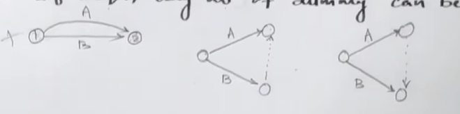
-
Looping (Cycling): This is a very important aspect of network diagrams. You do not want a loop/cycle in a network diagram. That's a problem.
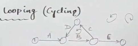
As we can see here, this network diagram has a loop in it, which violates the property of the activity, that the edge always flows from left to right, since here, activity C and D are flowing from right-to-left.
-
Fulkerson's Rule(Numbering the events): This is a very important rule that's applied when we want to number the events are the diagram is drawn.
So, if you have a preceding event
and succeeding event which has an activity of : That means that the preceding event's number will always be lesser than the succeeding event.
So, if we try to number the previous network diagram that had a loop in it:
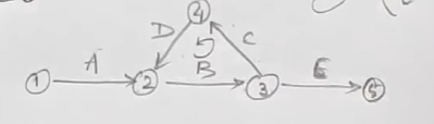
We can see that fulkerson's rule is being clearly violated, as an event with a bigger number is succeeded by an event with a smaller number (from node 4 to node 2).
However in all the other nodes, from events 1 to 2, 2 to 3, 3 to 4, and 3 to 5, fulkerson's rule is being followed.
Precedence Relationships
https://www.youtube.com/watch?v=3oONEQVsZPw&list=PLhSp9OSVmeyJKg_QaMV6qQdcGTFp2SbUH&index=3
-
Immediate Predecessor: Activities that must be completed immediately before another activity can start.
-
Dependencies: The order in which activities must be performed.
- Dependent tasks: Must wait for other tasks to complete.
- Concurrent tasks: Can be done in parallel.
Project Network Diagram
This is the important part. It's a network diagram showing:
- Nodes: Represent events (start/end points of activities).
- Arrows: Represent activities with durations.
- Direction: Shows precedence relationships.
Example 1: Drawing a basic network diagram.
https://www.youtube.com/watch?v=gJ4YsgDRr8g&list=PLhSp9OSVmeyJKg_QaMV6qQdcGTFp2SbUH&index=5
With all this information in mind, let's create a basic network diagram first, to familiarize ourselves with the process, before we proceed to any advanced methods like CPM or PERT.
So let's say we have a list of activities like this:
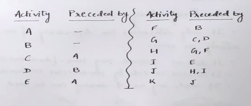
So we see that the starting activities are A and B, since they are preceded by none.
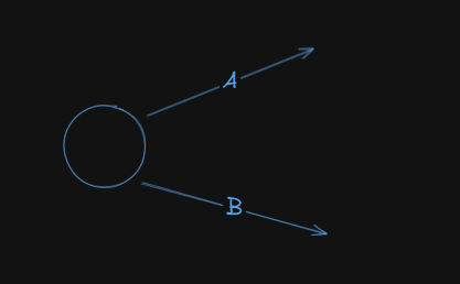
Next up, we have:
Activity C preceded by A
Activity E preceded by A
Activity D preceded by B
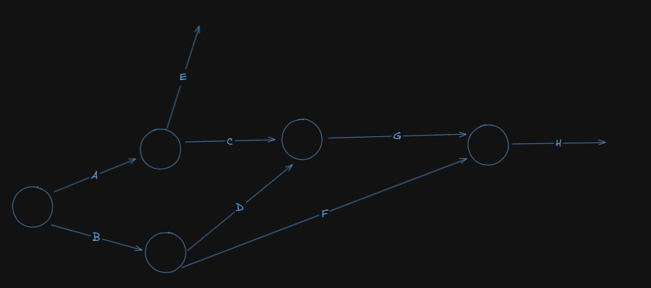
Now our network diagram looks like this:
Next up we have:
Activity F preceded by B
Activity G preceded by activities C and D
Activity H followed by activities G and F
So, our network diagram becomes:
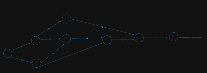
Next up, we have:
Activity I preceded by E
Activity J preceded by H and I
Activity K preceded by J
So, our network diagram becomes:
Now, let's number the events using fulkerson's rule:
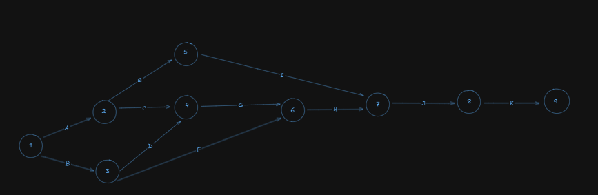
Note that I have added an ending event, which is node number 9 to mark the end of all the activities.
Important: If you have more than one ending nodes, coming from different activities, always merge them so that you always have a single ending node.
Critical Path Method (CPM)
Important Terminologies
Critical Path: The longest path through the network from start to finish. Activities on this path have zero slack - any delay causes project delay.
Earliest Start Time (EST): The earliest an activity can begin, assuming all predecessors are completed.
Earliest Finish Time (EFT): EST + activity duration.
Latest Start Time (LST): The latest an activity can start without delaying the project.
Latest Finish Time (LFT): The latest an activity can finish without delaying the project.
Slack/Float: How much an activity can be delayed without delaying the project:
With these terminologies in mind, let's solve an example to fully cement the understanding
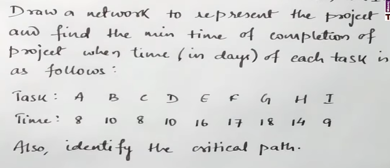
Example
https://www.youtube.com/watch?v=-Eguq6FAFH8&list=PLhSp9OSVmeyJKg_QaMV6qQdcGTFp2SbUH&index=8

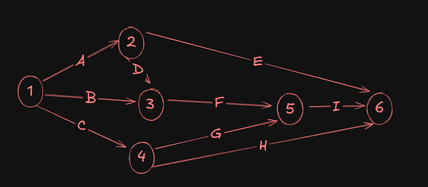
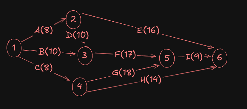
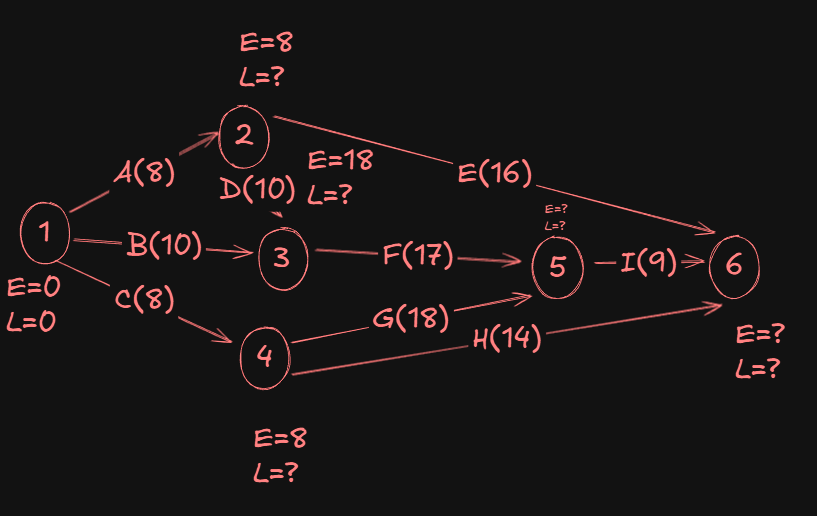
So we have this network diagram.
Let's get started on creating that first.
Now let's focus on the second part of the problem:
Now we have to add the time values for each activity in the network diagram:
Next, we will have to find the following for the network diagram:
- Earliest Start Time (EST)
- Latest Finish Time (LFT)
For this, we will augment all the nodes with two parameters, E, and L respectively.
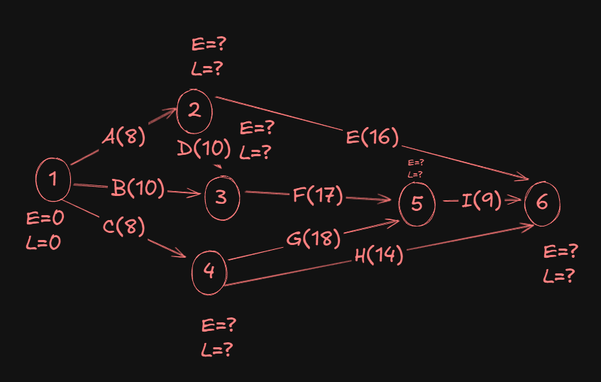
To update the E values first, we will use something called "Forward-Pass computation"
For this, we initially set E and L of the first node to zero.
Now as we proceed from the start to end (or source to sink), for the E values of each successor node, we will obtain the value by adding the E value of the previous node with duration of the activity preceding the successor node.
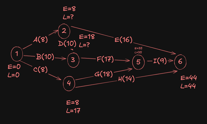
So for event 2, the E value will be 0 + 8 = 8, since 8 was the duration of the preceding activity A.
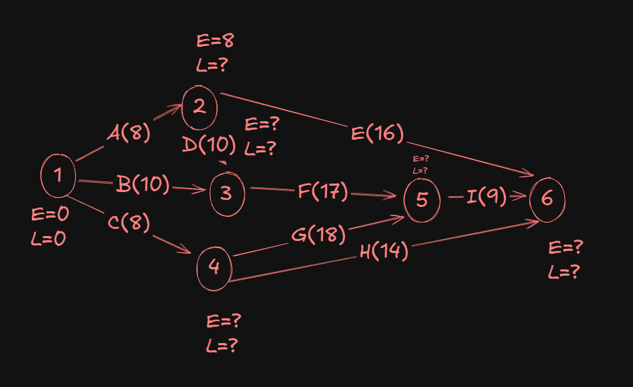
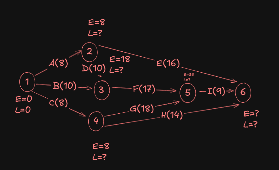
Now for event 3, we have two incoming activities, one from event 2 and the other from event 1.
In the event of multiple incoming activities on an event (node), we need to take the Max() of them to find the maximum value. This behaviour is reversed while finding L, when we take the Min().
Coming from 1->3 we would have the value of E as 0 + 10 = 10.
And coming from 2->3, we would have the value of E as 8 + 10 = 18.
A Max(10,18) gives us 18.
So the E value for event 3 will be 18.
For event 4, we would just get a 0 + 8 = 8.
Now for event 5:
- From
3->5we get18 + 17 = 35. - From
4->5we get8 + 18 = 26.
Max(35,26) gives us 35.
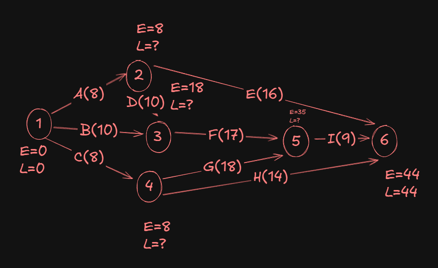
For event 6:
- From
2->6we have8 + 16 = 24 - From
5->6we have35 + 9 = 44 - From
4->6we have8 + 14 = 22
A Max(24,44,22) gives us 44.
Now, let's start finding the L values.
We start at the sink and trace back to the source, using something called Backward-pass computations. It's the same as what we did just now, but the reverse.
We start by setting the L value of the sink as the same as the E value.
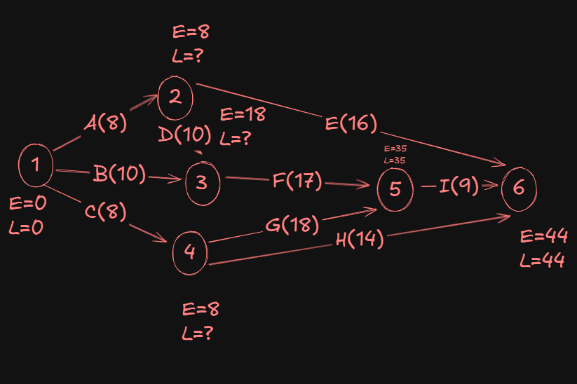
For event 5:
- From
6->5we have:44 - 9 = 35(yes we subtract now.)
Since that's the only activity edge connecting events 5 and 6, the L value of event 5 is 35.
For event 4:
- From
5->4we have35 - 18 = 17. - From
6->4we have44 - 14 = 30.
A Min(17, 30), gives us 17 as the L value of event 4.
Now, for event 3:
- From
5->3we have:35 - 17 = 18.
Since that's the only activity edge connecting events 3 and 5, the L value of event 3 is 18.
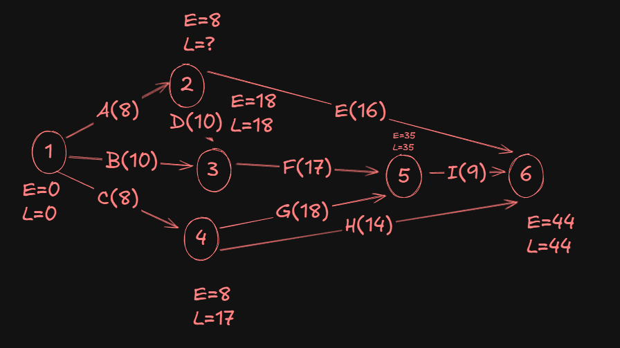
For event 2:
- From
6->2we have:44 - 16 = 28. - From
3->2we have:18 - 10 = 8.
A Min(28,8) gives us 8 as the L value of event 2.
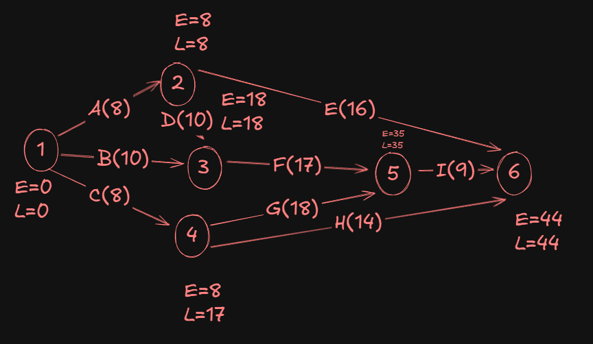
Now since I had already assumed the L value of event 1 as zero, it's written there, but for consistency purposes we will calculate the L value of event 1 again to check if there are any discrepancies.
So, for event 1:
- From
2->1, we have8 - 8 = 0. - From
3->1, we have18 - 10 = 8. - From
4->1, we have17 - 8 = 9.
A Min(0,8,9) gives us 0 as the L value of event 1.
So that remains unchanged then.
Hence our final network diagram:
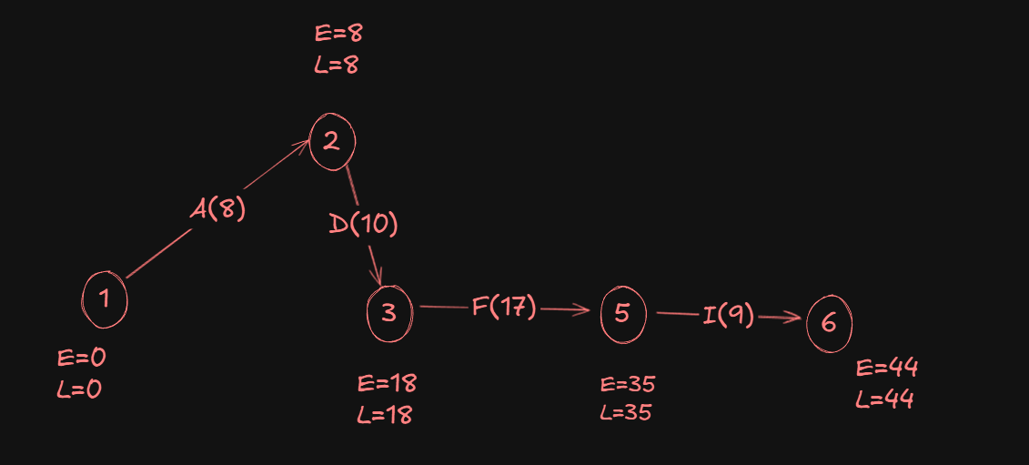
Finding the Critical Path.
To trace the critical path, the nodes we pick must obey the following rules:
Evalue equals to theLvalue for the head event (starting event).Evalue equals to theLvalue for the tail event(ending event)..
Following those rules, our critical path becomes:
PERT (Program Evaluation and Recommendation Technique)
Important terminologies
- Optimistic time estimate (
) - Most likely time estimate (
) - Pessimistic time estimate
- Order =
- Expected activity duration:
The edges will usually be given in the network diagram like this:
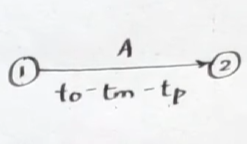
which can be converted by finding
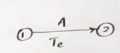
Standard deviation,
Variance
Example
https://www.youtube.com/watch?v=4xEzGAVEbR0&list=PLhSp9OSVmeyJKg_QaMV6qQdcGTFp2SbUH&index=13
Let's try to better understand how PERT works with the help of an example.
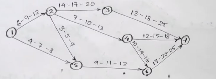
First, we quickly make a table like this:
| Activity | |||||
|---|---|---|---|---|---|
1->2 |
|||||
1->5 |
|||||
2->3 |
|||||
2->4 |
|||||
2->5 |
|||||
3->7 |
|||||
4->7 |
|||||
4->6 |
|||||
5->6 |
Next, we start filling up the values of each
| Activity | |||||
|---|---|---|---|---|---|
1->2 |
6 | 9 | 12 | ||
1->5 |
4 | 7 | 8 | ||
2->3 |
14 | 17 | 20 | ||
2->4 |
7 | 10 | 13 | ||
2->5 |
3 | 5 | 9 | ||
3->7 |
13 | 18 | 25 | ||
4->7 |
12 | 15 | 18 | ||
4->6 |
10 | 14 | 16 | ||
5->6 |
9 | 11 | 12 | ||
6->7 |
17 | 20 | 25 |
After that, finding the variance and expected time is just a matter of simple math.
| Activity | |||||
|---|---|---|---|---|---|
1->2 |
6 | 9 | 12 | 1 | 9 |
1->5 |
4 | 7 | 8 | 0.44 | 6.7 |
2->3 |
14 | 17 | 20 | 1 | 17 |
2->4 |
7 | 10 | 13 | 1 | 10 |
2->5 |
3 | 5 | 9 | 1 | 5.33 |
3->7 |
13 | 18 | 25 | 4 | 18.33 |
4->7 |
12 | 15 | 18 | 1 | 13.67 |
4->6 |
10 | 14 | 16 | 1 | 15 |
5->6 |
9 | 11 | 12 | 0.25 | 10.83 |
6->7 |
17 | 20 | 25 | 1.78 | 20.33 |
And there we have it, the variance and expected time for each activity.
Inventory Control: Economic Order Quantity (EOQ)
I don't even know why this topic is in this unit.
What is Economic Order Quantity?
Economic Order Quantity, also known as EOQ, is a widely used inventory management technique that helps organizations determine the optimal level of order quantity for a particular item, which minimizes the total inventory costs. The primary goal of EOQ is to provide a balance between the costs associated with ordering and holding inventory efficiently.
Formula for calculating Economic Order Quantity
Here,
- D is the demand for the product (in units) over a given period.
- S is the ordering cost per order.
- H is the holding cost per unit per year.
How does Economic Order Quantity Work?
Economic Order Quantity (EOQ) is an inventory management system that works by helping the organization determine the optimal order quantity for a particular item, inventory, or raw material. EOQ helps in balancing the costs associated with ordering and holding inventory to minimize the costs for the organization.
Here's how EOQ works in practical terms,
1. Units Consumed During the Year (A): The organization has to determine the annual demand for the product. This is the anticipated quantity of the product that the business is expected to use or sell in a year.
2. Ordering Costs (O): The organization has to determine and calculate the cost incurred each time an order is placed. The major chunks of costs include administrative, transportation, and other incidental costs related to the inventory or raw material procurement process.
3. Holding Costs or Carrying Cost (C): The organization has to determine the annual holding cost per unit of inventory. This includes all incidental costs like warehousing, insurance, security, and the opportunity cost of tying up capital in inventory.
4. Unit Cost: The organization should know the cost of each unit of inventory.
Once all the factors are analyzed, EOQ will help out the organization by providing the optimum level of inventory or raw material that shall be ordered, where both the carrying and ordering costs of inventory shall be the lowest.
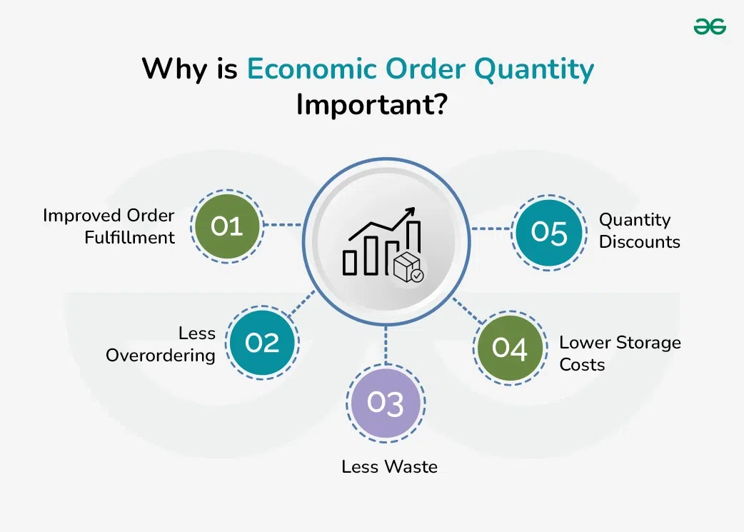
Why is Economic Order Quantity Important?
1. Improved Order Fulfillment: When a business is in need of a certain item or inventory to procure an order, an optimal level of EOQ ensures the product is on hand, which in turn helps the organization get the order out on time and cater to customer needs. This helps to enrich the customer experience and lead to increased sales.
2. Less Overordering: An accurate forecast about an organization's total consumption and when the organization will be in need of it helps the management avoid overordering and deploying too much working capital in inventory.
3. Less Waste: More optimized order schedules help an organization cut down on obsolete inventory, particularly for businesses that are engaged in holding perishable inventories, as it can result in dead stock and waste.
4. Lower Storage Costs: When the ordering matches the actual demand of the organization, it helps to process the optimal level of inventory to store, avoiding related costs like utility, security, insurance, and other related costs.
5. Quantity Discounts: When an organization properly plans and times the inventory or raw material, it allows the organization to take advantage of the best bulk orders or quantity discounts offered by the suppliers.
Example
Calculate the EOQ from the available particulars,
- Consumption of material per annum: 10,000kg
- Cost of making an order: ₹25
- Cost of raw material per kg: ₹5
- Storage cost: 10% on average inventory
D = Unit Consumed = 10,000
S = Ordering Cost = ₹25
H = Inventory Carrying Cost= 10% of 5 = ₹0.5
Therefore,
Here, the EOQ = 1000 Kg, which represent the optimum size of an order where the carrying cost and ordering cost will be minimum.