Module 3 -- Game Theory
Index
- Introduction to Game Theory
- Key terms
- 3. Maximin Strategy (Player A - Maximizing Player)
- 4. Minimax Strategy (Player B - Minimizing Player)
- 5. Saddle Point
- Understanding Practically
- Example 2 A Zero Sum Game where there is a saddle point
- The Graphical Method of solving
and games. - Example 1
case. - Example 2
case - Principle of Dominance
- Partial Dominance
- 🎯 Game Theory — Reasoning Trace (Complete Solving Guide) -- Final Summary.
Introduction to Game Theory
1. What is Game Theory?
Game theory studies conflict and cooperation between intelligent decision-makers. In OR, we focus on 2-person zero-sum games where:
- Two players compete
- One player's gain = Other player's loss
- Total payoff = 0
Example: Chess, poker, military strategy
Key terms:
| Term | Meaning |
|---|---|
| Player | Decision-maker (e.g., company, firm, individual). |
| Strategy | A complete plan of action under all situations. |
| Payoff | Outcome (gain/loss) from a particular combination of strategies. |
| Payoff Matrix | A table showing payoffs for all combinations of strategies. |
| Zero-sum game | One player’s gain = the other player’s loss. (Total = 0) |
| Non-zero-sum game | Total payoff ≠ 0 (both can gain or lose). |
2. Payoff Matrix
A matrix showing Player A's payoffs for all strategy combinations
           Player B
           B₁    B₂    B₃
Player A
   A₁     a₁₁   a₁₂   a₁₃
   A₂     a₂₁   a₂₂   a₂₃
   A₃     a₃₁   a₃₂   a₃₃
- Rows = Player A's strategies
- Columns = Player B's strategies
- Values = A's gain (B's loss)
3. Maximin Strategy (Player A - Maximizing Player)
Player A wants to maximize their minimum gain.
Steps:
- Find minimum in each row (worst case for A in that row)
- Select the row with maximum of these minimums
- This is Player A's maximin strategy
Maximin Value = max(row minimums)
4. Minimax Strategy (Player B - Minimizing Player)
Player B wants to minimize their maximum loss (or minimize A's maximum gain).
Steps:
- Find maximum in each column (worst case for B in that column)
- Select the column with minimum of these maximums
- This is Player B's minimax strategy
Minimax Value = min(column maximums)
5. Saddle Point
A saddle point exists when:
At the saddle point:
-
Element is minimum in its row (best for A against B's strategy)
-
Element is maximum in its column (best for B against A's strategy)
If saddle point exists:
- Game has a pure strategy solution
- Value of game = value at saddle point
- Both players should use their pure strategies
Understanding Practically
All that hit you all at once? Yeah, same here.
So, let's slow down, and understand with an example.
Step 1: Understanding the setup
We have two players:
We have two players:
-
A → the row player → wants to maximize their gain.
-
B → the column player → wants to minimize A’s gain (since B’s loss = A’s gain).
That’s why it’s called a zero-sum game:
whatever A gains, B loses equally.
The game is represented as a payoff matrix — payoffs to A.
Example (general form):
| a | b | |
| c | d |
Step 2: Formula for
If no saddle point exists, we use:
where:
Step 3: Example 1 -- Finding Saddle Point
Let's take this example:
| 2 | 4 | |
| 3 | 1 |
A wants to maximize, so first check worst-case for each row:
Before we proceed, let's understand the philosophy here.
Both players are rational and risk-aware:
- each tries to maximize their guaranteed gain and
- simultaneously minimize their possible loss.
So the logic is symmetric — just mirrored:
-
A: “Whatever B does, I want to make sure I’m not left with something too small.”
-
B: “Whatever A does, I want to make sure I don’t lose too much.”
That’s precisely what “maximin” and “minimax” capture.
Let's assume that B moves first. (Column access)
So assuming that B goes first, and tries to stop A from getting the higher value, but it doesn't know which row A will go for first.
Say, it goes with column
Going with the maximin rule that B follows, if B's thinking would be already grab the highest value per column and limit A to a "lower higher value", then B would already try to lock down the maximum, which is 4.
Now, with column
Now B looks at those worst cases (3 and 4) and picks the smaller one to limit A’s win:
This way, B can ensure A never earns more than 3.
Now in the next turn, A moves.
A assumes B will always pick the column that hurts A most (smallest in the row).
So for
So A already becomes pessimistic per row and gets the minimum value per row.
If that's the case then the maximin rule fits here perfectly since for
Similarly, for row
Now:
This way, A can guarantee itself at least 2.
Checking for saddle point.
As we know:
A saddle point exists when:
We have:
They don’t coincide → no saddle point → the game is unstable under pure strategies.
So, both must mix their choices probabilistically to reach equilibrium.
Step 4: Solve using formulae
From the payoff matrix:
| 2 | 4 | |
| 3 | 1 | |
| Here, |
Now, we apply the formulae:
So, the probability of
The probability of
And
Step 5: Interpretation
-
Since there was no saddle point, both players must randomize their choices.
-
On average, A will win 2.5 units per game if both play optimally.
-
If one player deviates, the other can exploit it to their advantage.
Example 2: A Zero Sum Game where there is a saddle point
| 4 | 1 | |
| 3 | 2 |
Same as before:
Step 1: Find A's row minima
A knows B will always pick the worst column (smallest value) in whatever row A chooses.
- Row
→ = 1 - Row
→ = 2
Now, taking a maximum of those minima:
So A can guarantee at least 2, no matter what B does.
Step 2: Find B's column maxima
B knows A will always pick the best row (largest value) in whatever column B chooses.
- Column
= 4 - Column
= 2
Now, taking a minimum of those maxima:
So B can limit A’s gain to at most 2.
Step 3: Compare to check if saddle point exists or not
✅ They coincide!
That means we’ve found a saddle point.
Step 4: Identify Saddle Point cell.
It’s the cell where the values of both the maximin and the minimax (2) appear in the matrix:
| 4 | 1 | |
| 3 | 2 |
So the saddle point is at the intersection of
Step 5: Interpretation.
- A’s optimal strategy → play A₂ every time.
- B’s optimal strategy → play B₂ every time.
- Value of the game
.
No mixing or probability needed — this pair (
If either player deviates, they’ll get a worse outcome.
The Stability Intuition
At the saddle point:
-
A can’t improve by switching rows (because B’s choice B₂ already gives them their best guarantee).
-
B can’t improve by switching columns (because A₂ already limits A’s maximum).
It’s literally like a saddle shape if you imagine the payoff as a surface:
-
It’s max along A’s direction (rows)
-
It’s min along B’s direction (columns)
That’s why the term saddle point is used.
The Graphical Method of solving
Why do we use the graphical method?
When:
- There is no saddle point, and
- The game is 2 x n (A has 2 strategies) or m x 2 (B has 2 strategies)
because in these cases, one variable (probability) can be plotted easily on a 2D graph.
Example 1:
Let's understand this better with the help of an example.
Given game:
| 2 | 4 | 6 | |
| 5 | 3 | 2 |
Step 1: What we're trying to find
- A is the row player (wants to maximize their payoff).
- B is the column player (wants to minimize A’s payoff).
Since there's no saddle point,
Let:
Step 2: Expected payoff for A
For each of B’s choices, we find A’s expected payoff (depending on p).
That will be as follows:
for each column
where each
Each of these is a linear equation in
They represent the payoff A will receive if B sticks to that strategy.
Now, from the payoff matrix:
| 2 | 4 | 6 | |
| 5 | 3 | 2 |
So, now we have three linear equations:
Plotting the equations.
- X-axis:
(ranging from 0 to 1) - Y-axis: Expected payoff
(based on the values of )
So the table would be as follows:
| Line | Equation | (E(p=0)) | (E(p=1)) |
|---|---|---|---|
| B₁ | (5 - 3p) | 5 | 2 |
| B₂ | (3 + p) | 3 | 4 |
| B₃ | (2 + 4p) | 2 | 6 |
Now that we have two points per line, we can draw them and find out the intersection points.
Using the concepts of Module 1 -- Basic Linear Programming Problems (LPP) and Applications#Topic 4 Graphical Method of Solving Linear Programming Problems we can plot a diagram and find the intersection points in the diagram between the lines as follows:
This is the graph.
Now, we need to find the intersection points of all the lines, pairwise.
Solving for:
So, now that we have the probability values, the expected payoffs for each value will be:
- At
:
- At
- At
Getting the envelope values per expected payoffs
Since we are working of A, who follows the maximin rule, first we will take a minimum for all 3 columns of all the expected payoffs.
Now the maximum of these envelope values is 3.5, which is at
That's the final answer, the optimal point,
Example 2:
Now B (the column player) has 2 strategies,
and A (the row player) has m strategies.
Let’s make it concrete with a 3×2 game (just enough to visualize).
| 2 | 6 | |
| 4 | 3 | |
| 5 | 1 |
These are the payoffs to A.
Step 1 — What we need to find
We want:
- B’s probability
: the chance B plays B₁ - (so
is ) - The value of the game
— A’s expected payoff when both play optimally.
Step 2 — Formula for expected payoff per row
For each row (A’s strategy),
the expected payoff to A, given B plays with probability q, is:
That’s the same pattern as earlier, just flipped.
Step 3 — Plug values for each row
| 2 | 6 | |
| 4 | 3 | |
| 5 | 1 |
| Row | Formula | Simplified Form |
|---|---|---|
What these mean
Each equation tells you how A’s expected payoff changes as B varies its strategy between B₁ and B₂.
- The first (6 - 4q) slopes down as q increases.
- The second (3 + q) slopes up slowly.
- The third (1 + 4q) slopes up fast.
Plotting the equations
If you were to plot this:
- X-axis →
(0 to 1) - Y-axis →
(expected payoff)
You’d get three lines:
| q | E(A₁) | E(A₂) | E(A₃) |
|---|---|---|---|
| 0 | 6 | 3 | 1 |
| 1 | 2 | 4 | 5 |
Visually:
-
A₁ starts highest (6) → goes down to 2
-
A₂ starts mid (3) → goes up to 4
-
A₃ starts low (1) → goes up to 5
-
A wants the payoff as high as possible.
-
B wants the payoff as low as possible.
So, for any given q:
-
A will choose the row that gives the maximum E (the topmost line).
-
B’s “effective” payoff to A is that maximum value (since A can always switch to the highest).
Find the intersection points
For:
(a)
(b)
(c)
Expected payoff values per equation:
| Row | Formula | Simplified Form |
|---|---|---|
For:
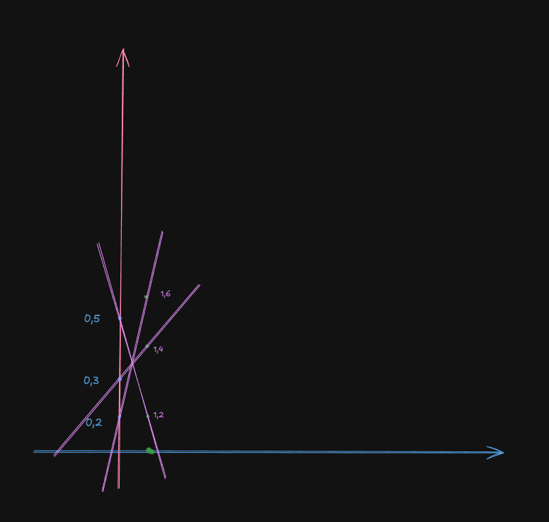
Finding the upper envelope values
Since we are working for B here, who follows the minimax rule, we will first find the maximum out of all the payoff values to find the 3 upper envelope values:
| q | E(A₁) | E(A₂) | E(A₃) | Upper envelope (max of rows) |
|---|---|---|---|---|
| 0.6 | 3.6 | 3.6 | 5.6 | 5.6 |
| 0.67 | 3.32 | 3.67 | 3.68 | 3.68 |
| 0.625 | 3.5 | 3.625 | 3.5 | 3.625 |
Now taking the minimum of this would get us
The probability of
Principle of Dominance
The principle of dominance is a shortcut to simplify large game matrices.
It says: if one strategy is always worse than another, it will never be chosen — so we can eliminate it from the matrix.
It’s like pruning unnecessary branches in decision making.
The idea, in simple words
For A (the maximizing player)
-
Each row belongs to A — it’s one of A’s possible strategies.
-
To check if a row is dominated, look at its cell values one by one.
-
If every cell in this row has a value less than or equal to the corresponding cell of another row (and at least one is strictly less),
→ the row is dominated and can be removed.
In short:
“If one row’s numbers are all smaller than another row’s numbers, the smaller row is useless — A will never play it.”
For B (the minimizing player)
-
Each column belongs to B — it’s one of B’s strategies.
-
To check if a column is dominated, compare its cell values vertically.
-
If every cell in this column is ==greater than or equal to ==the corresponding cell of another column (and at least one strictly greater),
→ that column is dominated and can be removed.
In short:
“If one column’s numbers are all bigger than another column’s numbers, the bigger column is useless — B will never play it.”
⚙️ Example 1 — Row dominance (A’s case)
| 2 | 4 | 3 | |
| 3 | 5 | 4 |
Compare cell by cell between A₁ and A₂:
A₂’s cells (3, 5, 4) are all greater than A₁’s (2, 4, 3).
→ A₂ dominates A₁ → remove A₁.
⚙️ Example 2 — Column dominance (B’s case)
| 4 | 6 | 5 | |
| 3 | 5 | 4 |
Compare cell by cell between B₂ and B₃:
B₃’s cells (5, 4) are both smaller than B₂’s (6, 5).
→ B₃ dominates B₂ → remove B₂.
Partial Dominance
Sometimes, no single row (or column) is completely better than another — but a combination of two (or more) strategies can produce values that are as good or better than another row or column in every cell.
That’s called partial dominance.
Case 1 — For A (maximizing player)
-
A’s strategies = rows.
-
Each row has several cell values.
-
If no single row dominates another, check whether a weighted mix of two rows (say, 50%-50% or any ratio) produces cell values that are all greater than or equal to another row’s cell values.
-
If yes, that “dominated” row can be removed.
In short:
“If mixing two of A’s rows gives cell values that are never smaller than another row’s values, that other row becomes useless.”
Example : A's partial dominance
| 4 | 3 | |
| 2 | 5 | |
| 3 | 4 |
No single row dominates A₃ directly.
But if A mixes A₁ and A₂ equally (50%–50%):
- B₁ → (4 + 2) / 2 = 3
- B₂ → (3 + 5) / 2 = 4
or:
| 3 | 4 | |
| 3 | 4 |
So this combination gives the pair (3, 4),
which is equal to or better than A₃’s (3, 4).
→ A₃ is partially dominated by the combination of A₁ and A₂ → remove A₃.
✅ Result: A₃ is redundant — A can achieve everything it does using a mix of A₁ and A₂.
Example: B's partial dominance
| 3 | 6 | 4 | |
| 4 | 2 | 3 |
No single column dominates another.
Now test if combining B₁ and B₂ (say, 50% each) gives smaller cell values than B₃.
Combination (B₁, B₂ → average):
- A₁ → (3 + 6) / 2 = 4.5
- A₂ → (4 + 2) / 2 = 3
| 4.5 | 4 | |
| 3 | 3 |
Compare with B₃ → (4, 3)
→ For A₁: 4.5 > 4 ❌ (slightly worse)
→ For A₂: 3 = 3 ✅
So this mix doesn’t dominate B₃ yet — but if we tweak the ratio (maybe 40%–60%), we might get smaller values for both rows.
If such a ratio exists, then B₃ would be partially dominated by (B₁, B₂).
The idea, simplified
| Player | Comparing what | What you’re checking | When to remove |
|---|---|---|---|
| A (maximizer) | Compare all cell values of one row vs mix of other rows | If every cell from the mix ≥ every cell in the row | Remove that row |
| B (minimizer) | Compare all cell values of one column vs mix of other columns | If every cell from the mix ≤ every cell in the column | Remove that column |
Practical Tip
You rarely need to calculate the exact mixing ratio in exams.
Usually, the question either gives you an obvious equal-weight example (like 50%-50%) or you just need to show that such a combination exists logically — not solve for it exactly.
🎯 Game Theory — Reasoning Trace (Complete Solving Guide) -- Final Summary.
🧩 1. Identify what type of game you’re solving
-
Check if the problem says two-person zero-sum game → use these steps.
-
Check the size of the payoff matrix:
- 2×2 → use saddle point or mixed strategy formulas.
- 2×n or m×2 → use graphical method.
- larger → apply principle of dominance first to reduce.
⚙️ 2. Check for Saddle Point (Pure Strategy)
-
For each row, find its minimum cell value (A assumes B minimizes).
-
Find the maximum of these minima → A’s Maximin.
-
For each column, find its maximum cell value (B assumes A maximizes).
-
Find the minimum of these maxima → B’s Minimax.
-
If Maximin = Minimax, saddle point exists:
- That value = Value of the Game (V).
- The corresponding cell = equilibrium point.
- ✅ Stop here — no mixing needed.
🧮 3. If No Saddle Point → Apply the Principle of Dominance
-
For A (row player):
Compare all cell values per row.
If every cell in one row is less than or equal to the corresponding cell in another row,
→ remove that row (it’s dominated). -
For B (column player):
Compare all cell values per column.
If every cell in one column is greater than or equal to the corresponding cell in another column,
→ remove that column (it’s dominated). -
Partial dominance:
If a combination of two rows (or columns) produces cell values that are never worse than another,
remove the dominated one. -
Repeat until no more rows or columns can be removed.
-
If reduced to 2×2 → go to Step 4.
⚙️ 4. 2×2 Game — Mixed Strategy Formula
Let the matrix be:
| B₁ | B₂ | |
|---|---|---|
| A₁ | a | b |
| A₂ | c | d |
Then use:
where:
= probability that A plays = probability that B plays = value of the game
Check that
If not, a pure strategy dominates and that row/column can be removed.
📈 5. 2×n Game — Graphical Method (A mixes)
-
Let A play
with probability and with . -
For each of B’s strategies (each column):
-
Plot
vs (p on x-axis, E on y-axis). -
The lowest line at each p shows what B can enforce (the lower envelope).
-
The highest point on that lower envelope = optimal point.
At that point:
= optimal probability for A. - The y-value at that intersection =
, the value of the game.
📉 6. m×2 Game — Graphical Method (B mixes)
-
Let B play
with probability and with . -
For each of A’s strategies (each row):
-
Plot
vs (q on x-axis, E on y-axis). -
The highest line at each q shows what A can get (the upper envelope).
-
The lowest point on that upper envelope = optimal point.
At that point:
= optimal probability for B. - The y-value at that intersection =
, the value of the game.
🧠 7. Interpretation
- If there’s a saddle point → that strategy pair is the equilibrium.
- If mixed → use the probabilities
and found from formulas or graphs. - The value of the game
represents: → A’s expected gain (B’s loss). → A’s expected loss (B’s gain).
🪶 8. Sanity Check Before Final Answer
- Are
and between 0 and 1? - Does
logically fit the data (no negative values if not expected)? - If dominance was applied, confirm that removed rows/columns truly made no difference.
- For graphs, make sure the intersection used lies on the active envelope (lower or upper as applicable).
✅ Short Mental Checklist
1️⃣ Write payoff matrix (for A).
2️⃣ Find Maximin and Minimax.
3️⃣ If equal → Saddle → Done.
4️⃣ Else → Apply Dominance.
5️⃣ If 2×2 → Use Formula.
6️⃣ If 2×n or m×2 → Use Graphical Method.
7️⃣ Read, , and , interpret results.