Module 4 -- Queueing Theory

#Operations-Research #Semester-7

Index

What is Queueing Theory?
Case 1 M/M/1 (∞ / FIFO) Poisson Queueing Model.
Example 1 (Infinite capacity)
Example 2 (Infinite capacity)
Case 2 M/M/1(N/FIFO)-- finite capacity queueing model
Key symbols/reminder
Two cases
Example 1 $p < 1$ case. (finite capacity)
Example 1 $p < 1$ case. (finite capacity)
M/M/1 (∞) vs M/M/1 (N) — Formula Comparison Table

What is Queueing Theory?

Queueing theory is all about understanding systems where “customers” arrive, wait, get served, and leave.
Customers can be people, packets, jobs, tasks — anything that “queues”.

Now we all know what a queue is.

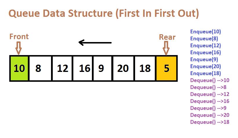
A queue is a linear data structure that follows the First-In, First-Out (FIFO) principle, meaning the first item added to the queue is the first one to be removed. Items are added to the rear of the queue (called enqueue) and removed from the front (called dequeue), much like people waiting in a line for a service.

Pasted image 20251113124859.png

So, what's with the new stuff then? Queueing Models, Poisson, $λ$ , $L$ , etc? Why do we need all this?

Case 1: M/M/1 (∞ / FIFO) Poisson Queueing Model.

Step 1: The need for Queueing Models

Think of queues in real life.
Are arrivals perfectly regular?

❌ No — people don’t arrive at exactly one every 10 seconds.
They come randomly: sometimes 2 people at once, sometimes no one for a minute.

Queueing Theory models random arrivals and random service times.

To describe randomness mathematically, we use a standard tool:

Poisson process → a way to model random arrivals.

And it uses one simple symbol:

$λ$ (lambda) -- the average arrival rate

If $λ = 10/hour \to$ on average, 10 customers arrive every hour.
Not exactly every 6 minutes — but on average.

That’s it. No magic.

Step 2: Service time is also random

You cannot serve every customer in exactly 5 minutes.
Sometimes 4, sometimes 7, etc.

So, we define:

$μ$ -- the average service rate

If $μ = 12 /hour \to$ server can serve 12 customers per hour on average.

Again — nothing complicated.

Step 3: Why do we need utilization?

This is the most intuitive part.

Utilization just means:

How busy is the server?

This is answered by this formula:

p = \frac{λ}{μ}

Example:

$λ = 10$ arrivals/hour
$μ = 12$ services/hour

Thus, $p = \frac{10}{12} = 0.833$ , the server is busy $83.3 %$ of the time.

Now,

If $λ \geq μ$ , this means that customers arrive faster than they can be served, which makes the queue grow to infinity and the system breaks.

So the only condition for a working queue is:

$μ > λ$
(server must be faster than arrivals)

Step 4: The M/M/1 Queueing Model

M/M/1 literally means:

M → arrivals follow a Markovian (Poisson) process
M → service times are Markovian (exponential distribution)
1 → one server

You do not need to study distributions deeply.
All you need to accept is:

Poisson arrivals + exponential service = simplest realistic queue model.

Step 5: Important Terminologies

These are just average quantities:

L = average number of customers in the whole system
(waiting + being served)
$L_{q}$ = average number waiting in the queue
W = average time a customer spends in the system
$W_{q}$ = average time spent waiting in the queue

They are connected by the famous but simple:

Little's law

L = λ W

If more customers arrive per hour, L increases.
If each customer spends more time in the system, L increases.
Simple.

Formula set for M/M/1 (∞ / FIFO)

Let $λ$ be the arrival rate (customers per hour), $μ$ be the service rate (customers per hour), $p = \frac{λ}{μ}$

Stability condition: $λ < μ$
Utilization: $p = \frac{λ}{μ}$
Probability that the system is empty: $P_{0} = 1 - p$
Probability of $n$ customers in system: $P_{n} = (1 - p) \times p^{n}$
Average number of customers in the system $L = \frac{p}{(1 - p)}$
Average number of customers waiting in queue: $L_{q} = \frac{p^{2}}{1 - p}$
Average time in system: $W = \frac{1}{μ - λ}$
Average waiting time in queue: $W_{q} = \frac{p}{(μ - λ)}$

Whoops. Too many formulae? Hell nah I myself am not memorizing all that, so let's simplify all this with the core formulae that we can use to build all these.

We need to remember 3 rules and 2 definitions.

Definition 1: $λ$ is the arrival rate of customers per hour.
Definition 2: $μ$ is the service rate of customers per hour.

Rule 1: The utilization of the server is given by the ratio of the arrival rate to the service rate of the customers per hour. (Or the average number of customers that are being served.)

Just “how busy the server is”.

Thus:

p = \frac{λ}{μ}

Now, for the probability that the system is empty, we can just get the value by subtracting it from 1:

P_{0} = 1 - p = μ - λ

Then, the probability of $n$ customers in system becomes:

P_{n} = P_{0} \times p^{n} = (1 - p) \times p^{n}

Rule 2: Average number of customers in the system (This means the people waiting in the queue plus the one person that is being served (if there is one)). This one formula unlocks everything else.

Intuition:
If the server is almost full most of the time, L becomes large.
If server is fast compared to arrivals, L stays small.

L = \frac{p}{(1 - p)}

Rule 3: Little's Law!

L = λ W

From here we can get the average time in system $W$ :

W = \frac{L}{λ}

or:

W = \frac{\frac{p}{(1 - p)}}{λ}

W = \frac{\frac{\frac{λ}{μ}}{(1 - \frac{λ}{μ})}}{λ}

W = \frac{\frac{λ}{μ - λ}}{λ}

W = \frac{λ}{λ (μ - λ)}

W = \frac{1}{μ - λ}

Now, for the average number of customers waiting in queue ( $L_{q}$ ):

We go back to the definition of L first:

L is the average number of customers in the system (This means the people waiting in the queue plus the one person that is being served (if there is one))

So,:

L = average waiting + average in service

or:

L = L_{q} + average in service

Fair so far. We are halfway there.

Now, for the average customers that is in service.

We know that the average number of customers that are being served is defined by $p$ .

But why, a probability? Why $p$ ?

In an M/M/1 queue, the number of customers being served is either:

0 (server idle) (Let's take is as $P_{i d l e}$ )
1 (server busy) ( $P_{b u s y}$ )

There is no other possibility.

So, the average number of customers in service become:

p (or p_{t o t a l}) = 0 \times p_{i d l e} + 1 \times p_{b u s y}

So, there we have $p$ as the average number of customers that are being served. And the probability that there are no customers and the server is idle is $P_{0} = 1 - p$ . Simple.

So,

average in service = p

Plugging this back into our earlier structure:

L = L_{q} + p

L_{q} = L - p

L_{q} = \frac{p}{(1 - p)} - p

L_{q} = \frac{p - p + p^{2}}{(1 - p)}

Finally:

L_{q} = \frac{p^{2}}{(1 - p)}

Lastly, for the average waiting time in queue $W_{q}$ :

This one is very symmetrical to $W = \frac{L}{λ}$ from Little's law:

W_{q} = \frac{L_{q}}{λ}

W_{q} = \frac{\frac{p^{2}}{(1 - p)}}{λ}

W_{q} = \frac{p^{2}}{λ (1 - p)}

Substituting $λ = p μ$ ,

W_{q} = \frac{p^{2}}{p μ (1 - p)}

W_{q} = \frac{p}{μ - μ \frac{λ}{μ}}

Finally:

W_{q} = \frac{p}{μ - λ}

Example 1

Given arrival rate $λ$ is 8 customers per hour, and the service rate $μ$ is 12 customers per hour.

Find:

Utilization rate of the server.
Probability that the server is empty.
Probability of 1 customer in the system.
Average number of customers in the system.
Average waiting time per customer in the queue.
Average time spent in system.
Average waiting time in the queue.

Solution:

(a) The utilization:

p = \frac{λ}{μ} = \frac{8}{12} = 0.66

(b) Probability that the server is empty (not being utilized):

1 - p = 1 - 0.66 = 0.34

P_{1} = (1 - p) p^{n} = (1 - p) p = 0.66 \times 0.34 = 0.2244

(d) Average number of customers in the system:

L = \frac{p}{(1 - p)} = \frac{0.66}{0.34} = 1.941

(e) Average waiting time of customers in the queue:

L_{q} = \frac{p^{2}}{(1 - p)} = \frac{0.4356}{0.34} = 1.281

(f) Average time spent in the system:

From Little's law

L = λ W ⟹ W = \frac{L}{λ}

W = \frac{1.941}{8} = 0.242

(g) Average waiting time in the queue:

W_{q} = \frac{L_{q}}{λ}

W_{q} = \frac{1.281}{8} = 0.1601

Short interpretation: server busy 66.7% of the time; on average 2 customers in system (1.333 waiting + 0.666 being served); each customer spends 15 min total, waiting 10 min.

Example 2

Given average waiting time in queue $W_{q} = \frac{1}{6}$ hours or $W_{q} = 0.166$ hours, the service rate $μ = 6$ customers/hours,

Find:

Arrival rate of customers.
Utilization rate of the server.
Probability that the server is empty.
Average number of customers in the system.
Average waiting time per customer in the queue.
Average time spent in system.

(a) The arrival rate of customers:

From:

W_{q} = \frac{p}{μ - λ}

and:

p = \frac{λ}{μ}

W_{q} = \frac{λ}{μ^{2} - μ λ}

λ = W_{q} μ^{2} - W_{q} μ λ

λ + W_{q} μ λ = W_{q} μ^{2}

λ (1 + W_{q} μ) = W_{q} μ^{2}

λ = \frac{W_{q} μ^{2}}{(1 + W_{q} μ)}

λ = \frac{0.166 \times 36}{1 + (0.166 \times 6)}

λ = \frac{5.976}{1 + 0.996}

λ = \frac{5.976}{1.996}

λ = 2.993 \approx 3 customers per hour

(b) Utilization rate:

p = \frac{λ}{μ} = \frac{3}{6} = 0.5

P_{0} = 1 - p = 0.5

(d) Average number of customers in the system:

L = \frac{p}{(1 - p)} = \frac{0.5}{0.5} = 1

(e) Average waiting time of customers in the queue:

L_{q} = \frac{p^{2}}{(1 - p)} = \frac{0.25}{0.5} = 0.5

(f) Average time spent in the system:

From:

L = λ W

W = \frac{L}{λ}

W = \frac{1}{3} = 0.33

Interpretation: with those numbers, arrivals are half the service rate; average one customer in system (0.5 waiting, 0.5 in service); customers wait 10 minutes on average and spend 20 minutes total.

Case 2: M/M/1(N/FIFO)-- finite capacity queueing model

Short plain-English first: now the system can hold at most N customers (including the one in service).

If an arrival finds $N$ customers already present, that arrival is blocked (lost). Everything else (Poisson arrivals, exponential service, FCFS), stays the same.

Key symbols/reminder

$λ$ = offered arrival rate
$μ$ = service rate
Utilization, $p = \frac{λ}{μ}$
$N$ = system capacity (max customers including one in service)
$P_{n}$ = steady-state probability of $n$ customers in the system ( $0 \leq n \leq N$ )
$λ_{e f f} = λ (1 - P_{N})$ = accepted arrival rate (use this in Little’s Law for times)

Two cases

$p = 1$ , arrivals exactly equal to service

For the infinite M/M/1 queue, we reject ρ≥1 because the queue would blow up.

For the finite case, the queue cannot blow up, it's capped at $N$ . So even if arrivals = service i.e. $p = 1$ , the system stays stable because arrivals beyond $N$ are rejected.

So, when $p = 1$ ,

P_{n} = P_{0} \times p^{n} = P_{0} (1^{n}) = P_{0}

All probabilities become equal.

But we still need them to sum to 1:

P_{0} + P_{1} + \dots + P_{N} = 1

That's:

(N + 1) P_{0} = 1

P_{0} = \frac{1}{N + 1}

P_{n} = \frac{1}{N + 1}, n = 0, 1, \dots, N

And for $p < 1$ it's all the more acceptable since the arrivals are slower than the service system, so the system stays stable.

Numerical solving.

Alright now since I am pressed for time, I will stop with the theoretical explanations here and skip ahead to how to solve numericals of the finite case using only 4 formulae.

One master formula:

Utilization for $n$ customers:

P_{n} = \frac{p^{n}}{\sum_{k = 0}^{N} p^{k}}

One arrival formula:

Effective arrival:

λ_{e f f} = λ (1 - P_{N})

One average formula

Average number of customers in the system

L = \sum_{n = 0}^{N} n P_{n}

Little's law (same as infinite queue case)

W = \frac{L}{λ}

and:

W_{q} = \frac{L_{q}}{λ_{e f f}}

and:

L_{q} = L - (1 - P_{0})

Example 1: $p < 1$ case.

Given arrival rate = 3 customers per hour, service rate = 5 customers per hour and max system capacity = 4 customers.

Find:

Utilization
Utilization for all customers ranging from none (system empty) to the max system capacity ( $N$ )
The effective arrival
Average number of customers in the system
Average waiting time of customers in the queue
Average time spent in the system
Average time spent in the queue

So, we have:

$λ = 3$
$μ = 5$
$N = 4$

(a) Utilization:

ρ = \frac{3}{5} = 0.6

(b) Utilization for all customers ranging from none (system empty) to the max system capacity ( $N$ ):

From:

P_{n} = \frac{p^{n}}{\sum_{k = 0}^{N} p^{k}}

Computing the denominator first:

\sum_{k = 0}^{4} {0.6}^{k} = p^{0} + p^{1} + p^{2} + p^{3} + p^{4}

\sum_{k = 0}^{4} {0.6}^{k} = 1 + 0.6 + 0.36 + 0.216 + 0.1296 = 2.3056

So,

P_{n} = \frac{{0.6}^{n}}{2.3056}

$P_{0} = \frac{1}{2.3056} = 0.4336$
$P_{1} = \frac{0.6}{2.3056} = 0.2601$
$P_{2} = \frac{0.36}{2.3056} = 0.1561$
$P_{3} = \frac{0.216}{2.3056} = 0.09365$
$P_{4} = \frac{0.1296}{2.3056} = 0.05619$

The blocking probability is $P_{N} = P_{4} = 0.05619$ i.e. the probability of utilization of the server when any further arrivals in the queue will be lost/rejected.

λ_{e f f} = λ (1 - P_{N})

λ_{e f f} = 3 (1 - P_{4}) = 3 (1 - 0.05619)

λ_{e f f} = 2.8314

(d) Average number of customers in the system:

L = \sum_{n = 0}^{N} n P_{n}

Here $n$ starts from zero and proceeds till $N$ times.

So,

L = \sum_{n = 0}^{4} n P_{n} = 0 \cdot P_{0} + 1 \cdot P_{1} + 2 \cdot P_{2} + 3 \cdot P_{3} + 4 \cdot P_{4}

L = 0 + 0.2601 + 2 (0.1561) + 3 (0.09365) + 4 (0.05619)

L = 1.07796

(d) Average time spent waiting by customers in the queue:

L_{q} = L - (1 - P_{0}) = 1.07796 - (1 - 0.4336)

L_{q} = 1.07796 - 0.5664

L_{q} = 0.51156

(e) Average time spent in the system:

W = \frac{L}{λ_{e f f}}

W = \frac{1.07796}{2.8314} = 0.3807 hr

(f) Average time spent in the queue:

W_{q} = \frac{L_{q}}{λ_{e f f}}

W_{q} = \frac{0.51156}{2.8314}

W_{q} = 0.1807 hr

Example 2: $p = 1$ case

Given arrival rate = 4 customers per hour, service rate = 4 customers per hour and max system capacity = 3 customers.

Find:

Utilization
Utilization for all customers ranging from none (system empty) to the max system capacity ( $N$ )
The effective arrival
Average number of customers in the system
Average waiting time of customers in the queue
Average time spent in the system
Average time spent in the queue

So, we have:

$λ = 4$
$μ = 4$
$N = 3$

(a) Utilization:

ρ = \frac{4}{4} = 1

(b) Utilization for all customers ranging from none (system empty) to the max system capacity ( $N$ ):

From:

P_{n} = \frac{p^{n}}{\sum_{k = 0}^{N} p^{k}}

Computing the denominator first:

\sum_{k = 0}^{3} 1^{k} = p^{0} + p^{1} + p^{2} + p^{3}

\sum_{k = 0}^{4} 1^{k} = 1 + 1 + 1 + 1 + = 4

So,

P_{n} = \frac{1^{n}}{4}

$P_{0} = \frac{1}{4} = 0.25$
$P_{1} = \frac{1}{4} = 0.25$
$P_{2} = \frac{1}{4} = 0.25$
$P_{3} = \frac{1}{4} = 0.25$

The blocking probability is $P_{N} = P_{3} = 0.25$ i.e. the probability of utilization of the server when any further arrivals in the queue will be lost/rejected.

λ_{e f f} = λ (1 - P_{N})

λ_{e f f} = 4 (1 - P_{3}) = 4 (1 - 0.25)

λ_{e f f} = 3

(d) Average number of customers in the system:

L = \sum_{n = 0}^{N} n P_{n}

Here $n$ starts from zero and proceeds till $N$ times.

So,

L = \sum_{n = 0}^{3} n P_{n} = 0 \cdot P_{0} + 1 \cdot P_{1} + 2 \cdot P_{2} + 3 \cdot P_{3}

L = 0 + 0.25 + 2 (0.25) + 3 (0.25)

L = 1.5

(d) Average time spent waiting by customers in the queue:

L_{q} = L - (1 - P_{0}) = 1.5 - (1 - 0.25)

L_{q} = 1.5 - 0.75

L_{q} = 0.75

(e) Average time spent in the system:

W = \frac{L}{λ_{e f f}}

W = \frac{1.5}{3} = 0.5 hr

(f) Average time spent in the queue:

W_{q} = \frac{L_{q}}{λ_{e f f}}

W_{q} = \frac{0.75}{3}

W_{q} = 0.25 hr

M/M/1 (∞) vs M/M/1 (N) — Formula Comparison Table

Just as a final summary.

Concept	M/M/1 (Infinite capacity)	M/M/1 (Finite capacity, max = N)
Utilization	$ρ = \frac{λ}{μ}$	$ρ = \frac{λ}{μ}$
State probabilities	$P_{n} = (1 - ρ) ρ^{n}$	$P_{n} = \frac{ρ^{n}}{\sum_{k = 0}^{N} ρ^{k}}$
Probability of empty system	$P_{0} = 1 - ρ$	$P_{0} = \frac{1}{\sum_{k = 0}^{N} ρ^{k}}$
Blocking probability	Not applicable (no blocking)	$P_{N}$
Effective arrival rate	$λ_{eff} = λ$	$λ_{eff} = λ (1 - P_{N})$
Avg. number in system	$L = \frac{ρ}{1 - ρ}$	$L = \sum_{n = 0}^{N} n P_{n}$
Avg. number in queue	$L_{q} = \frac{ρ^{2}}{1 - ρ}$	$L_{q} = L - (1 - P_{0})$
Avg. time in system	$W = \frac{L}{λ} = \frac{1}{μ - λ}$	$W = \frac{L}{λ_{eff}}$
Avg. waiting time in queue	$W_{q} = \frac{L_{q}}{λ} = \frac{ρ}{μ - λ}$	$W_{q} = \frac{L_{q}}{λ_{eff}}$
Stability requirement	$λ < μ$ (must hold)	Always stable (capacity finite)
Little’s Law	$L = λ W$ , $L_{q} = λ W_{q}$	$L = \lambda_{\text{eff}} W $, $ L_q = \lambda_{\text{eff}} W_q$

Index

What is Queueing Theory?

Case 1: M/M/1 (∞ / FIFO) Poisson Queueing Model.

Step 1: The need for Queueing Models

λ (lambda) -- the average arrival rate

Step 2: Service time is also random

μ -- the average service rate

Step 3: Why do we need utilization?

Step 4: The M/M/1 Queueing Model

Step 5: Important Terminologies

Little's law

Formula set for M/M/1 (∞ / FIFO)

Example 1

Example 2

Case 2: M/M/1(N/FIFO)-- finite capacity queueing model

Key symbols/reminder

Two cases

p = 1, arrivals exactly equal to service

Numerical solving.

One master formula:

One arrival formula:

One average formula

Little's law (same as infinite queue case)

Example 1: p < 1 case.

Example 2: p = 1 case

M/M/1 (∞) vs M/M/1 (N) — Formula Comparison Table

$λ$ (lambda) -- the average arrival rate

$μ$ -- the average service rate

$p = 1$ , arrivals exactly equal to service

Example 1: $p < 1$ case.

Example 2: $p = 1$ case