Index

1. What is Mechanics?
2. 1. Constraints in Mechanics
3. 2. Friction
4. Laws of Friction (Empirical)
5. Basics of Vector Calculus.
6. 1. Gradient
7. 2. Divergence
8. 3. Curl
9. Line Integrals
10. Line Integral for scalar fields.
11. Line Integral for Vector Fields
12. Pre-requisite to Partial Differential Equations Ordinary Differential Equations
13. A very basic idea of Partial Differential Equations.
14. Potential Energy function.
15. Equipotential Surfaces
16. Conservative vs Non Conservative Forces
17. Conservation Laws of Energy and Momentum
18. Non-inertial frame of reference
19. Simple Harmonic Oscillator
20. Dampened harmonic motions and oscillations
21. Resonance (not the song)
22. Angular Velocity and it's vector
23. Moment of Inertia

What is Mechanics?

Mechanics is the branch of physics that deals with the motion of objects and the forces that cause that motion. It is divided into two main parts:

• Kinematics: Describes motion without considering its causes.
• Dynamics: Focuses on the forces and their effects on motion.

Let's break down the first topic step by step.

1. Constraints in Mechanics

What are Constraints?

In mechanics, a constraint is a condition that restricts the motion of a particle or a system. It limits the degrees of freedom (the number of independent ways in which the system can move).

Example

Let's dive into a simple and easy to understand example

Imagine a small bead threaded onto a fixed circular wire of radius $R$. The bead can move freely on the wire, but it cannot leave the wire.

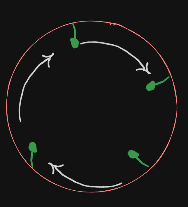
1. Free Particle in 2D

• If the bead were completely free on a flat plane, it would have two coordinates: $x$ and $y$.

• It could move anywhere, so it has 2 degrees of freedom.

2. Adding the Constraint

• Now, the bead must always be on the circle: $x^2+y^2=R^2$.

• This equation is a constraint: it links $x$ and $y$ together.

3. Physical Meaning

• Bead can no longer move independently in both $x$ and $y$—for any chosen $x$, $y$ must satisfy the constraint.

• So, only one degree of freedom remains: you can describe the position using a single variable, say the angle $\theta$ (measured from a reference direction).

4. Expressing in Terms of Constraint

• Position of the bead: $x=Rcos\theta$, $y=Rsin\theta$ (polar coordinates)
• As $\theta$ changes, the bead moves on the circle, but always satisfies : $x^2+y^2=R^2$.

Types of Constraints:

• Holonomic Constraints: Relations expressible as equations involving coordinates and possibly time (e.g., a particle must stay on a circle: ($x^2+y^2=R^2$).

• Non-Holonomic Constraints: Not integrable into equations of coordinates only (e.g., rolling without slipping).

Mathematical Representation:

Suppose you have $N$ particles in 3D space; their coordinates are ($x_i,y_i,z_i$) for $i=1,2,...,N$

• Without constraints, total degrees of freedom = $3N$.

• Each holonomic constraint reduces degrees of freedom by one.

2. Friction

What is Friction?

I am going to assume that you have been out of touch with physics for years on end, and need a total recap.

Friction is the "stickiness" or "grabbiness" between two surfaces that touch each other. It's what makes it hard to slide things around.

Real-Life Examples:

• When you try to push a heavy box across the floor, it resists moving – that's friction!

• When you rub your hands together, they feel warm – that's friction creating heat!

• When you walk, your shoes grip the ground so you don't slip – that's friction helping you!

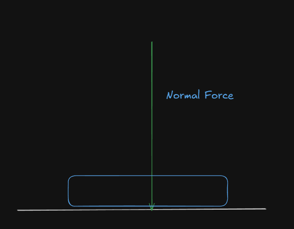
Normal Force (The "Pressing Together" Force)

Before we talk about friction laws, we need one simple concept:

Normal Force = How hard the two surfaces are pressed together

Examples:

• A book sitting on a table: the book's weight presses it against the table

• You pushing down on a box while trying to slide it: you're increasing how hard it's pressed against the floor

• A car going around a curve: the car is pressed against the road by its weight

Key Point: The harder you press two surfaces together, the more friction there will be between them.

Types of Friction:

1. Static Friction ($f_s$)(When Things Are NOT Moving)

This is the friction that prevents things from starting to move.

Real-life example: You push lightly on a heavy box, but it doesn't move. Static friction is holding it in place, matching your push exactly.

2. Kinetic Friction($f_k$) (When Things ARE Moving)

This is the friction that slows down things that are already sliding.

Real-life example: Once you push the box hard enough and it starts sliding, kinetic friction tries to slow it down and stop it.

Laws of Friction (Empirical):

Law 1: Static Friction Can Vary

• What it means: Static friction can be any value from zero up to a maximum

• Real-life: If you push a box gently, friction matches your push exactly (box doesn't move). Push harder, friction increases to match. But there's a limit!

• The limit: Maximum static friction = ${\mu }_s$ × (how hard surfaces are pressed together)

  • ${\mu }_s$ = "static friction coefficient" = a number that depends on what materials are touching

Law 2: Kinetic Friction is Constant

• What it means: Once something is sliding, the friction stays the same

• Real-life: Once the box starts sliding, the friction force stays constant (doesn't change with how fast it's sliding)

• The amount: Kinetic friction = μₖ × (how hard surfaces are pressed together)

  • ${\mu }_k$ = "kinetic friction coefficient" = usually smaller than μₛ

Law 3: Direction of Friction

• Simple rule: Friction always opposes motion (or attempted motion)

• Real-life: If you push right, friction pushes left. If something slides down a hill, friction tries to push it back up the hill.

A Simple Example

Scenario: You're trying to slide a 10 kg box across a wooden floor.

1. Light Push: You push with 20 N of force → Box doesn't move → Static friction = 20 N (opposing your push)

2. Harder Push: You push with 50 N → Box still doesn't move → Static friction = 50 N

3. Maximum Push: You push with 80 N → Box just starts to move → You've reached maximum static friction = 80 N

4. Box Sliding: Once moving, kinetic friction might be 60 N → Box slides but slows down due to this constant 60 N friction

3. Problems Involving Constraints & Friction

Let's combine the two concepts with a classic example:

Classic Exam Problem: Block on an Inclined Plane

A $5$ kg block sits on a rough inclined plane that makes a $30\text{°}$ angle with the horizontal. The coefficient of static friction is ${\mu }_s=0.6$ and kinetic friction is $\mu ₖ=0.4$.

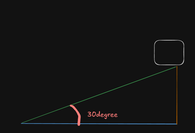
Questions:

1. Will the block slide down the plane?
2. If it slides, what is its acceleration?

Step 1: Identify the Constraint

The constraint here: The block must move along the inclined plane (it can't fly off or sink into the plane).

This means we only need to consider motion parallel to the plane (green line) and forces perpendicular to the plane (green line).

Step 2: Draw and Identify forces

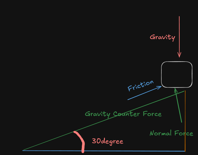
This diagram I drew, is called a Free body diagram (FBD) and it's a must for visualizing the problem better.

The forces acting on this block are:

• It's own weight (gravity) : $mg$ (let the acceleration due to gravity, $g$ be $10m/s^2$)
• The counter force to gravity (Newton's third law), also known as the normal force($N$), which is acting perpendicular from the surface of the plane.
• And the friction ($f$) on the surface of the plane, that will be acting against the sliding down of the block.

Step 3: Break down the weight into components

Since the plane is tilted, we split the weight:

• Component along the plane (trying to slide the block down, $y$ axis) : is given by this formula ($r\sin \theta$) or in this case, $r=mg$. So, that will be $5\times 10\cdot \sin 30\text{°}$ or $25$ N.

• Component into the plane (pressing the block against surface along the slope of the plane, $x$ axis): is given this formula : $r\cos \theta$ or in this case, $r=mg$. So that will be $5\times 10\cdot \cos 30\text{°}$ or $43.3$ N.

Step 4: Find the normal force

The normal force balances the component pressing into the plane (since it's acting perpendicular to the plane, it will be related to the $x$ axis):

Step 5: Calculate the maximum static friction

As we know, static friction is friction acting against the block when it is already at rest.

The formula for calculating the maximum static friction is :

where ${\mu }_s$ is the given static friction constant and $N$ is the normal force we just calculated.

So, the maximum static friction is $0.6\times 43.3=26N$

Step 6: Check if block will slide.

Now that we know how much friction is acting against the block, we can find out whether the block will slide or not by simply comparing the maximum static friction force against the gravitational pull acting on the block.

Gravitational pull experienced by the block is the vertical weight component (along the $y$ axis), which we just calculated to be 25 N.

Since, 25 N is obviously less than the frictional force of 26N, the block will not slide down.

Basics of Vector Calculus.

For the specific purpose of mechanics, we will be focusing on the first basics of vector calculus.

The partial derivatives chain rule:

https://www.youtube.com/playlist?list=PLF-vWhgiaXWNi9OuPCbguaPgL67XH7crm

You can refer to this playlist for a quick recap of the multivariable calculus chain rule (TheOrganiChemistryTutor math)

https://www.youtube.com/watch?v=XipB_uEexF0&list=PLF-vWhgiaXWNi9OuPCbguaPgL67XH7crm&index=3

A very simple method of solving a multivariable calculus equation via the chain rule is to draw a tree like this:

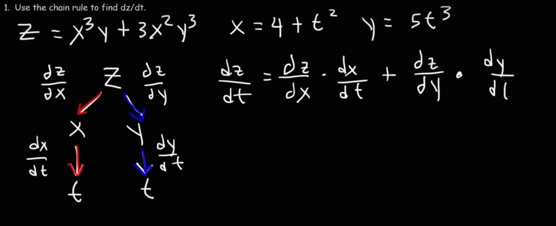
And once we have constructed the equation, we can then just perform standard differentiation rules to solve it.

1. Gradient

The gradient is an operation on a scalar field that produces a vector field. It indicates the direction and magnitude of the steepest increase of a function at a given point.

The gradient of a scalar field $f(x,y,z)$ is a vector field given by:

For a 2D scalar field, that would be : $\mathrm{\nabla }f=(\frac{df}{dx},\frac{df}{dy})$

A small example:

Let's say we have a scalar function:

We have to find it's gradient at points $1,-2,-1$

Finding each partial derivative:

Final gradient:

And the result, is a vector field.

2. Divergence

The divergence is an operation on a vector field that produces a scalar field. It measures the magnitude of a vector field's "source" or "sink" at a given point. A positive divergence indicates a source (fluid flowing outward), a negative divergence indicates a sink (fluid flowing inward), and a divergence of zero means there is no net flow in or out.

For a vector field $F=P\hat{i}+Q\hat{j}+R\hat{k}$

The divergence, $divF=\mathrm{\nabla }\cdot F=\frac{dP}{dx}+\frac{dQ}{dy}+\frac{dR}{dz}$

Example

Let's say we have a vector field as follows:

Let:

• $P=(x^{2}y)$
• $Q=(x^3)$
• $R=(z^2)$

So,

And the result is, that we now have a scalar field instead.

3. Curl

The curl is an operation on a vector field that produces another vector field. It measures the "circulation" or infinitesimal rotation of the field at a given point. The resulting vector's direction indicates the axis of rotation, and its magnitude represents the speed of rotation.

For a vector field $F=P\hat{i}+Q\hat{j}+R\hat{k}$,

The curl is given by this determinant:

which unfolds to:

Example

Let's say that we have a vector field: $F=(y)\hat{i}+(xz)\hat{j}+(x^2)\hat{k}$

Let:

• $P=(y)$
• $Q=(xz)$
• $R=(x^2)$

So the curl will be:

This vector field describes the rotational properties of the original vector field $F$.

Pre-requisites: Line Integrals of scalar and vector fields.

Integral calculus recap

https://www.youtube.com/watch?v=hXOrQ0Ao4UE&list=PLF-vWhgiaXWM7Iri0t_AjBfv51tF28PEy&index=1&pp=gAQBiAQB

The above link points to a full comprehensive recap of class 12 recap. Watch it only if you have time.

Following recap section taken from Integral Calculus#Class 12 level recap

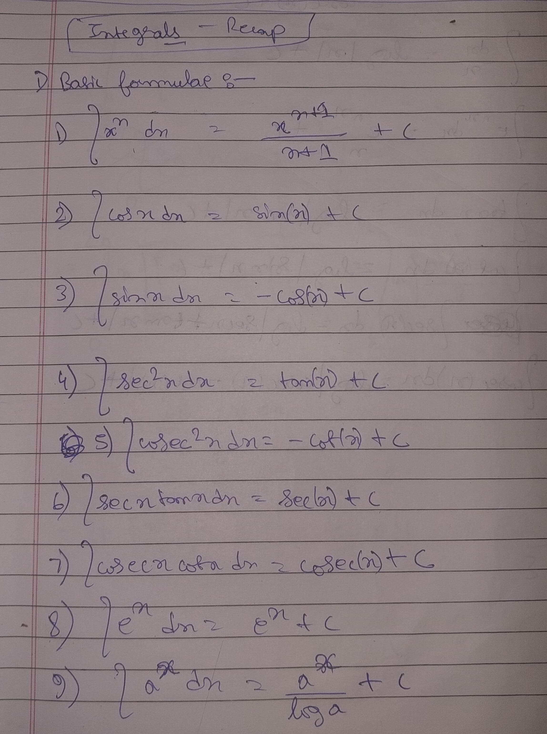
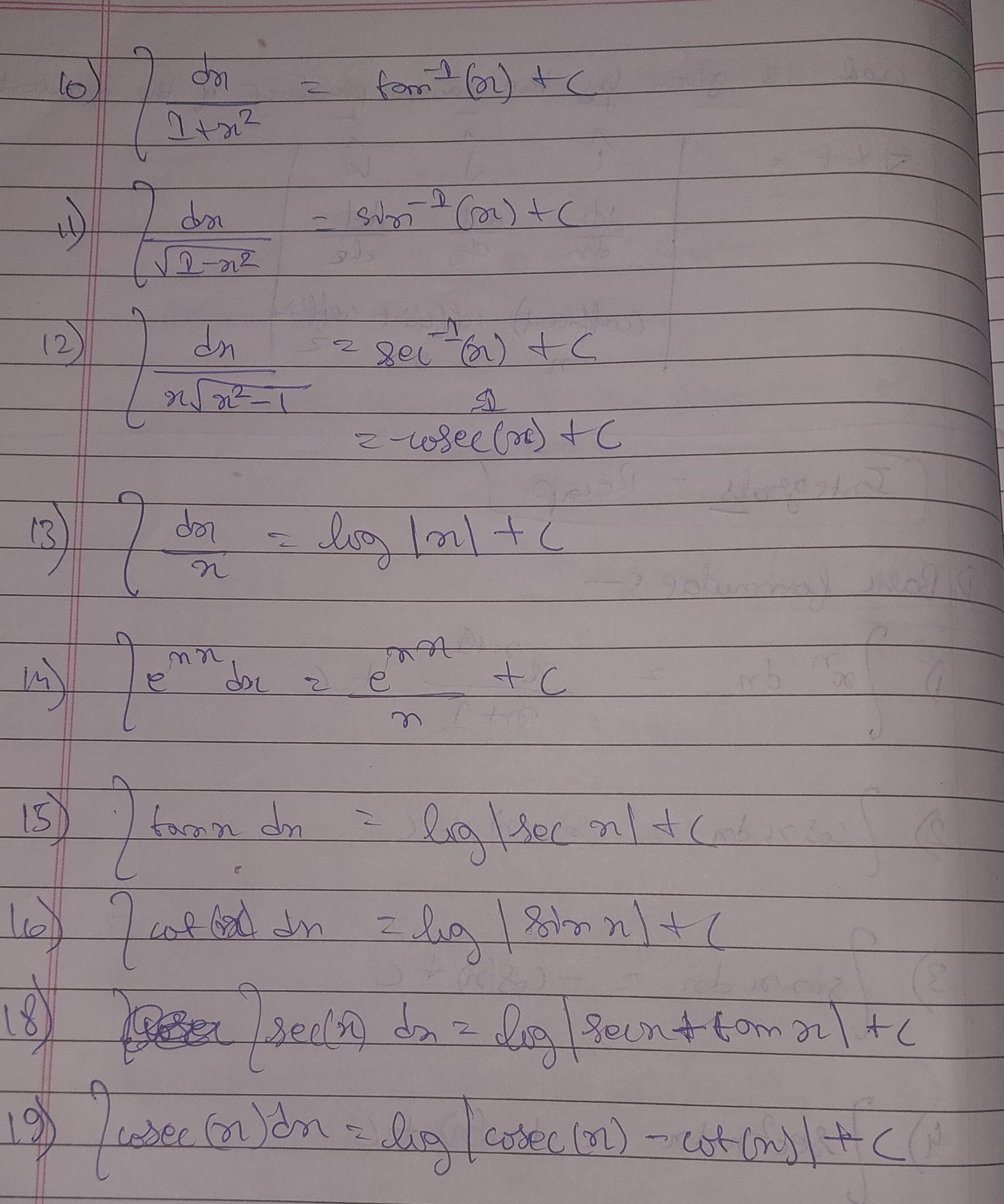
Basic Integral Formulae

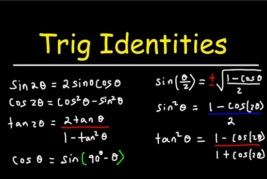
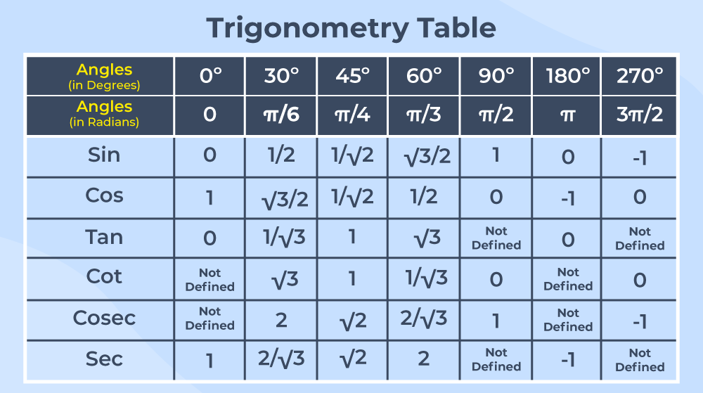
Some basic trigonometric identities

https://www.youtube.com/watch?app=desktop&v=m1OitPmkydY

https://www.geeksforgeeks.org/trigonometric-identities/

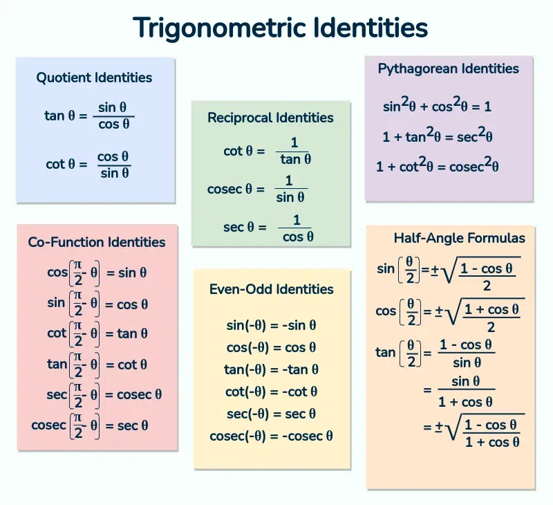
https://www.geeksforgeeks.org/trigonometry-table/

Methods of integration

1. U-substitution

So let's say we have an integral

To solve this using u-substitution, we need to:

1. set $x=g(t)$.
2. Differentiate both sides
3. So, we get : $${dx} = g'(t).dt$$
   And then we replace the value of $x$ and $dx$ in the original equation to get:

Example 1 :

1. $$\int sin(mx)dx$$

Let us set $mx=t$ and differentiate both sides w.r.t $x$, we get :

And thus we replace $dx$ in the original equation to get:

or , $$\frac{-cos(mx)}{m} + C$$

Example 2

Let $$1+x^2 = t$$

or $$\implies 0 + 2x = \frac{dt}{dx}$$
or, $$2x dx = dt$$
Replacing this in the original equation,

or ,

2. Integration by Parts -- The easy method.

https://www.youtube.com/watch?v=2I-_SV8cwsw&list=PLF-vWhgiaXWM7Iri0t_AjBfv51tF28PEy&index=2

This is called the D-I method. Differentiate-Integrate. (also known as the LIATE method)

Example 1.

So let's say we have this integral here :

We need to make a small table.

The D column represents differentiation and I column represents integration.

Now we choose each term to be either differentiated or integrated.

Here the easy choice seems to differentiate $x^2$ and integrate $sin(3x)$

Now we continue the respective operations on both sides for a while.

Each column having alternating signs.

What to differentiate and what to integrate?

• Inverse trigonometric functions (like $ta{n}^{-1}$, $si{n}^{-1}$) — differentiate these if present.
• Logarithmic functions (like ln(x)) — differentiate these if present.
• Algebraic functions (like $x^2$, $x$, constants) — differentiate these if no inverse or logarithmic terms are present.
• Trigonometric functions (like $sin(x)$, $cos(x)$) — differentiate these if there are no inverse, logarithmic, or algebraic terms to use.
• Exponential functions (like $e^x$, $a^x$) — these are typically integrated as a last choice.

When to stop the operations:

1. If the column of D reaches 0.
2. If the products of a row (product of both the value of D and I) can be integrated.
3. If any the products of any row (product of both the value of D and I) result in the original integral.

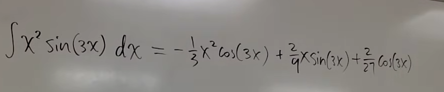
So here we see that the column of D has reached 0.

So we multiply downwards, diagonally, along with each respective sign, and write them together for the final answer.

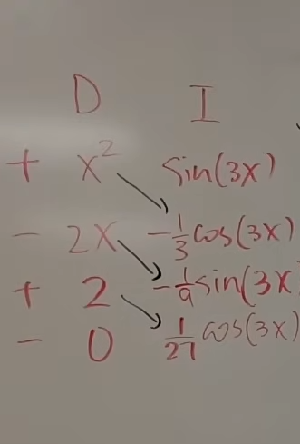
Like this.

So the final answer becomes,

Example 2

Let's say we have another integral

Example 3:

Let's say we have another integral, $$e^x.sin(x)dx$$

Remembering our rules, we differentiate $e^x$, since functions like $e^x$ are integrated as a last choice. And the remaining $sin(x)$ will be differentiated.

So ,

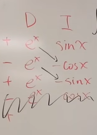
So we stop the operations and write diagonal products first.

or $$2\int{e^x.sin(x)dx} = e^{x}.[sin(x)-cos(x)]$$
or, $$\int{e^x.sin(x)dx} = \boxed{\frac{e^{x}.[sin(x)-cos(x)]}{2}}$$

3. Integration by partial fractions -- An easy method

https://www.youtube.com/watch?v=OFEfGtCsVKg&list=PLF-vWhgiaXWM7Iri0t_AjBfv51tF28PEy&index=4&pp=gAQBiAQB

This method can only be applied if the denominator can be factorized into linear factors

or that in denominator power of $x$ is 1, or it is a product of terms in which power of $x$ is 1.

Example 1

So let's say we have an integral :

We can see that it's denominator is in the form of a product of linear factors.

So the way to tackle this, is to take one term at a time.

We first select $(x-1)$.

Equate this term to 0. We get $x=1$.

Now we apply this value back in the original equation, but there's a twist.

We modify this part of the process by removing the selected term from denominator, but instead placing it in the form of a natural log (log or $ln$), and we don't substitute the value of $x$ in that log term.

1. So, for $(x-1)$

or $$\frac{-ln(x-1)}{6}$$
2. For $(x+2)$, we get $x=-2$

or $$\frac{2(-2) - 1}{(-2-1)(-2-3)}ln(x+2)$$

or $$\frac{-5.ln(x+2)}{15} = \frac{-ln(x+2)}{3}$$
3. For $(x-3)$, we get $x=3$.

or $$\frac{2(3) - 1}{(3-1)(3+2)}.ln(x-3)$$
or $$\frac{5.ln(x-3)}{10} = \frac{ln(x-3)}{2}$$
Finally we put all the obtained terms together along with their signs.

as our complete answer.

The given video link has another example on this.

Line Integrals

https://www.youtube.com/watch?v=dnGDmZynvYY (line integrals, for scalar and vector fields as well.)

If you happen to think that line integrals are regular, double or triple integrals, then you are mistaken.

Line integrals are NOT regular integrals, double integrals, or triple integrals. They are a completely different type of integral that integrates along a curve or path.

Regular Integrals vs Line Integrals

Regular integral: $\int f(x)dx$ (integrates over an interval on x-axis)
Double integral: $\int \int f(x,y)dxdy$ (integrates over a 2D region)
Triple integral: $\int \int \int f(x,y,z)dxdydz$ (integrates over a 3D region)

Line integral: ${\int }_{C}fds$ (integrates along a specific curve C in space)

Visual Difference

• Regular integral: Area under a curve

• Line integral: Sum of values along a path (like walking along a trail and adding up something at each step)

What does this mean?

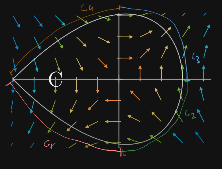
So let's say we divided the curve into 4 smaller "line curves" or just lines.

Naming them $c_1$, $c_2$, $c_3$, $c_4$, each.

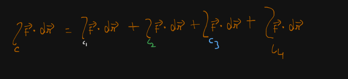
Now the LHS side, the "line integral of F over C" would be given by finding the line integrals of all the smaller line curves and summing them up.

So we would get : $$\boxed{\int_c{F} \ dr = \int_{c_1}{F} \ dr \ + \int_{c_2}{F} \ dr + \ \int_{c_3}{F} \ dr + \ \int_{c_4}{F} \ dr} $$
where the surface C is traversed in the counter-clockwise direction.

Line Integral for scalar fields.

Basically the exact same thing which I demonstrated above:

Simple Example: Mass of a Wire

Scenario: You have a curved wire in space, and the wire has varying density at different points.

Setup

• Wire follows a curve C (like a bent coat hanger)
• Density function: $\rho (x,y,z)=x^2+y^2$ (density increases as you move away from the origin)
• Question: What's the total mass of the wire?

Solution Process:

1. Break the wire into tiny pieces of length ds

2. At each piece:

   • Find the density $\rho$ at that point
   • Mass of tiny piece = $\rho \times ds$

3. Add up all tiny masses: Total mass = ${\int }_C\rho (x,y,z)$ ds

So let's say we divided the wire into 4 smaller "wire curves" or just wires.

Naming them $c_1$, $c_2$, $c_3$, $c_4$, each.

The total density would be:

Real-World Analogy:

Imagine walking along a trail where you pick up rocks. The "density" tells you how many rocks per meter you find at each location. The line integral gives you the total number of rocks collected.

Line Integral for Vector Fields

We can find the line integral for a vector field, let's say a curve in it, by taking the dot product of the curve plugged into the vector field function and the derivative of the curve.

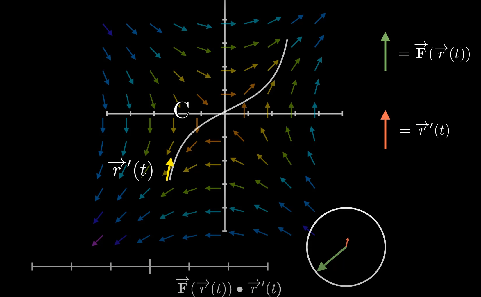
Let's try to understand this with a simple example.

Simple Example: Work Done by a Force

Scenario: You're pushing a box along a curved path through a force field.

Setup:

• Force field: F($x,y)=(y,-x)$ (imagine wind that swirls counterclockwise)

• Path C: You move the box from point (1,0) to (0,1) along a quarter circle

• Question: How much work does the force field do on the box?

Solution Process:

1. Break the path into tiny steps dr

2. At each step:

   • Find the force F at that point

   • Work done in tiny step = F · dr (dot product!)

   • This gives: (force in direction of motion) × (distance moved)

3. Add up all tiny work contributions: Total work = ∫_C F·dr

Pre-requisite to Partial Differential Equations: Ordinary Differential Equations

Differential equations recap from calculus-3 (semester 3)

Basic types of differential equations.

1. Linear Differential equation.

These can be of two types:

1. $$\boxed{{\displaystyle \frac{dy}{dx}+P(x).y=Q(x)}}$$

To solve this, we find an integrating factor(I.F).

And we find the solution in terms of y as:

2. $$\boxed{{\displaystyle \frac{dx}{dy}+P(y).x=Q(y)}}$$

Same stuff, just in terms of x this time.

I.F = $$I.F = e^{\int{P(y) dy}}$$

And we find the solution in terms of x as: $$\boxed{x . (I.F) = \int{Q(y) . (I.F) dy} + C}$$

2. Exact equations

An ordinary D.E of first order and first degree is of the form: $$\frac{dy}{dx} = F(x,y)$$ can be written as: $\boxed{{\displaystyle Mdx+Ndy=0}}$

This equation will be considered exact, if and only if

and the solution of the equation will be given by:

However there are times when :

and thus the equation by-default is not exact.

However we can convert it to an exact equation by finding an integrating factor and then multiplying it to the original equation.

Steps for finding integrating factor for a non-exact equation.

1. If equation is of the form $\boxed{{\displaystyle Mdx+Ndy=0}}$
2. Then check if $\frac{dM}{dy}\ne \frac{dN}{dx}$
3. If true, then equation is non-exact.

Proceeding from here:

Case 1

1. Check if both M and N are homogenous (degree of both the functions should be equal to zero).
2. If case 1 is true, then check if both M and N have same degree
3. If true, then check if $Mx+Ny\ne 0$ .
4. If all of the above are true, then the I.F will be: $$\boxed{\frac{1}{Mx + Ny}}$$
5. Multiply this I.F to the original equation to get the exact equation. Proceed solving from there as previously discussed.

Case 2 (M and N are both not homogenous/M is not homogenous/N is not homogenous)

1. In this case, we proceed by finding : $$\frac{dM}{dy} - \frac{dN}{dx}$$
2. Now we can either:
   1. Divide by M: If the result is a function of y and y only, then our I.F will be: $$\boxed{e^{-\int{g(y)dy}}}$$
   2. Divide by N: If the result is a function of x and x only, then our I.F will be: $$\boxed{e^{\int{f(x)dx}}}$$
3. Multiply this I.F to the original equation to get the exact equation. Proceed solving from there as previously discussed.

For the alternate form

1. If equation is of form $$\boxed{y(f(x,y)dx + xg(x,y)dy) = 0}$$
2. M = $y(f(x,y)$ , N = $xg(x,y)$.
3. If$$Mx-Ny\ne 0\$\$,then$$
4. Multiply this I.F to the original equation to get the exact equation. Proceed solving from there as previously discussed.

Second Order Differential Equations

We will mainly require this in future topics such as the harmonic oscillator (pendulum).

A linear D.E of second order with constant coefficients is of the form:

2
where $P_1$ and $P_2$ are constants and $X$ is either a constant or a function of $x$ itself.

We can solve this equation by first converting it to it's auxiliary form using the D-operator method.

Using the symbol D for the differential operator $\frac{d}{dx}$ , the above equation can be written as:

Case 1: Solving homogenous part and finding C.F

Now if $X$ is equal to zero then the equation becomes homogenous. To solve this we need to find a complementary factor or C.F.

Rules for finding Complementary factor, C.F

1. Convert the given differential equation to it's auxiliary form. For example :

2. Solve the equation and find it's two roots $m_1$ and $m_2$.

3. If the roots are different, the solution becomes:

   $$y=c_1.e^{m_1.x}+c_2.e^{m_2.x}$$

   where $c_1$ and $c_2$ are arbitrary constants.

4. If the roots are same, i.e $m_1=m_2$, then the solution becomes:

   $$y=[c_1+c_2.x]e^{mx}$$

5. If the roots are complex then, the solution becomes:

   $$y=e^{ax}[c_1.cos(bx)+c_2.sin(bx)]$$

   where $m=a+bi$ , $a=0$ , $b=1$.

   or $$y = c_1.cos(bx) + c_2.sin(bx)$$

Case 2: Solving the non-homogenous part of the differential equation.

In the event of : $$(D^2 + P_1D + P_2)y = X$$, $X$ is not a constant, there is a different way to find the solution to this equation.

Firstly we assume $y=e^{mx}$ to be a trial solution to this equation and find C.F for the homogenous part, and we write it down as :

Now for the non-homogenous part, we need to find something called a Particular-Integral or P.I.

The entire general solution will be

There are two ways to find the P.I .

Method 1: Using the inverse operator method (not really recommended in my opinion)

Let the non-homogenous D.E be :

We do this by setting :

Solving $(D^2+a_1.D+a_2)$ , we get either $(D-a{)}^n$ or $(D+a)$ or $(D-a)(D+b)$

Now a few important cases of $f(x)$ and formulae for those cases.

1. $$\frac{1}{(D-a)}.X=e^{ax}.\int X.e^{-ax}dx$$

2. $$\frac{1}{D}.X=\int Xdx$$

3. If you have :

   $$\frac{1}{(D-m_1)(D+m_2)}.X$$

   or

   $$\frac{1}{f(D)}.X$$

   , where $m_1$ and $m_2$ are roots of $f(D)$, then we can get the P.I as follows:

   $$\frac{1}{f(D)}=\frac{A_1}{D-m_1}+\frac{A_2}{D-m_2}$$

   which is solved as:

   $$\frac{1}{f(D)}.X=A_1.e^{m_1.x}.\int X.e^{-m_1.x}+A_2.e^{m_2.x}.\int X.e^{-m_2.x}$$

Now to find the values of $A_1$ and $A_2$.

Let's say we have a given expression

where $m_1=1$ and $m_2=-1$.

We can write

or

Cancelling out $x.e^{2x}$ from both sides and multiplying both sides by $(D-1)(D+1)$,

We get

or

Now we compare both the coefficient of $D$ and constant terms to the other side.

Since there is no $D$ on the other side, $(A+B)=0$, and $1$ is on the other side, so

$A-B=1=>A=B$

From the two equations, we get $A=\frac{1}{2}$ , $B=-\frac{1}{2}$

So we get our P.I as:

which, when solved completely, gives us:

as the solution for this P.I.

4. If you have :

   $$\frac{1}{f(D)}.X$$

   where $X=P(x)$, is a polynomial function of some degree $m$, we get the P.I as:

   $$[f(D){]}^{-1}.P(x)$$

   where we expand $D$ till $D^m$ and then solve $P(x)$.

5. If you have:

   $$\frac{1}{f(D)}.e^{ax}.V$$

   , where $V$ is a function of a $x$. We can get the solution as:

   $$P.I=e^{ax}.\frac{1}{f(D+a)}.V$$

Method 2: Using the method of variation of parameters.

This method is used when it's difficult to apply the inverse operator method. However it is not a replacement for the inverse operator method. Both are valid, usage depends on the question.

So picking up from our C.F for equation: $$(D^2 + P_1D + P_2)y = X$$

where we assumed the C.F to be: $$y = c_1.y_1(x) + c_2.y_2(x)$$
Now, let us assume our P.I as $$y = u.y_1(x) + v.y_2(x)$$, where $u$ and $v$ are unknown functions of $x$

To find the value of $u$ and $v$, we need to find the Wronskian Determinant, which is given by

and $$u' =
\begin{vmatrix}
0 \ y_2 \
X \ y'_2 \
\end{vmatrix}
= \frac{-y_2.X}{W}$$

and

or

and

Put these values back into your P.I equation to get the full general solution to the D.E

A very basic idea of Partial Differential Equations.

Unlike the normal differential equations, PDEs are an entirely different breed and are very hard to understand, and even solve, since there exists no systematic direct framework or list of formulae as we saw in the previous sections.

Hence, since it's mentioned in the syllabus, we will just explore a very brief idea as how PDEs work and where they are needed.

🔹 Step 1. The “why” of PDEs

Think of PDEs like this:

• An ODE (ordinary differential equation) says: “How does one variable change in time?”

• A PDE says: “How does something change when more than one variable is involved?”

Example:

• If I track your gym weight over time → ODE.
• If I track the temperature at different points in your room as time passes → PDE (because it depends on both space and time).

So a PDE is basically just an equation saying: “This function of many variables balances out in a certain way.”

🔹 Step 2. First simple PDE:

This means:
“The slope of $z$ with respect to $x$ plus the slope of $z$ with respect to $y$ is always zero.”

How to solve (intuition-first):

• Imagine you move in the $x$-direction → $z$ increases.
• To cancel that, if you move in the $y$-direction, $z$ must decrease by the same amount.

That suggests $z$ depends only on the difference between $x$ and $y$, not on them separately.

So we try $z(x,y)=f(x-y)$.

Check:

• Differentiate wrt $x$: $z_x=f\prime (x-y)$.

• Differentiate wrt $y$: $z_y=-f\prime (x-y)$.

• Add them: $f^{\prime }(x-y)-f^{\prime }(x-y)=0$. ✅ Works.

👉 So the “trick” is: look for a relationship that keeps things balanced. In this case, moving in $x$ and moving in $y$ had to cancel, so I guessed a function of $x-y$.

Now, we can usually better understand a relationship between the functions with the help of visualizations or diagrams.

But, PDEs are way harder to tame than ODEs, and that’s why they don’t have one nice neat “general formula.”

🔹 Why no single formula for PDEs?

• For linear ODEs, we have systematic methods (integrating factor, characteristic equations, etc.).
• For PDEs, the space of possible equations is much larger (different variables, orders, nonlinear terms, boundary conditions).

So instead of one universal formula, we have different toolkits:

• Separation of variables (good for symmetric, physics-y PDEs).
• Method of characteristics (good for first-order PDEs).
• Fourier transforms / series (good for periodic or infinite domains).
• Green’s functions, numerical methods… (for real-world stuff).

Your exam will not expect all that — just the very first steps.

And that's all that's needed for a very basic idea of PDEs

Potential Energy function.

In physics, be it any system, they always want to move from a higher to lower potential energy value, as this state is more stable and requires less external effort to maintain. For example, a ball rolls down a hill (high gravitational potential energy) to a lower point (low gravitational potential energy), and a positive electric charge moves from high to low electric potential.

Now, how can we find the best way to decrease a system from higher to lower potential energy?

Well, if you are someone like me who studied Machine Learning before physics, in Module 4 -- Sparse Modeling and Estimation, Modeling Time-Series Data, Deep Learning and Feature Representation Learning.#What is Gradient Descent? deep learning, you would that we use Gradient Descent method to minimize the cost function of a network, to "effectively nudge the system towards a desired pattern of weights and biases to get a desired output."

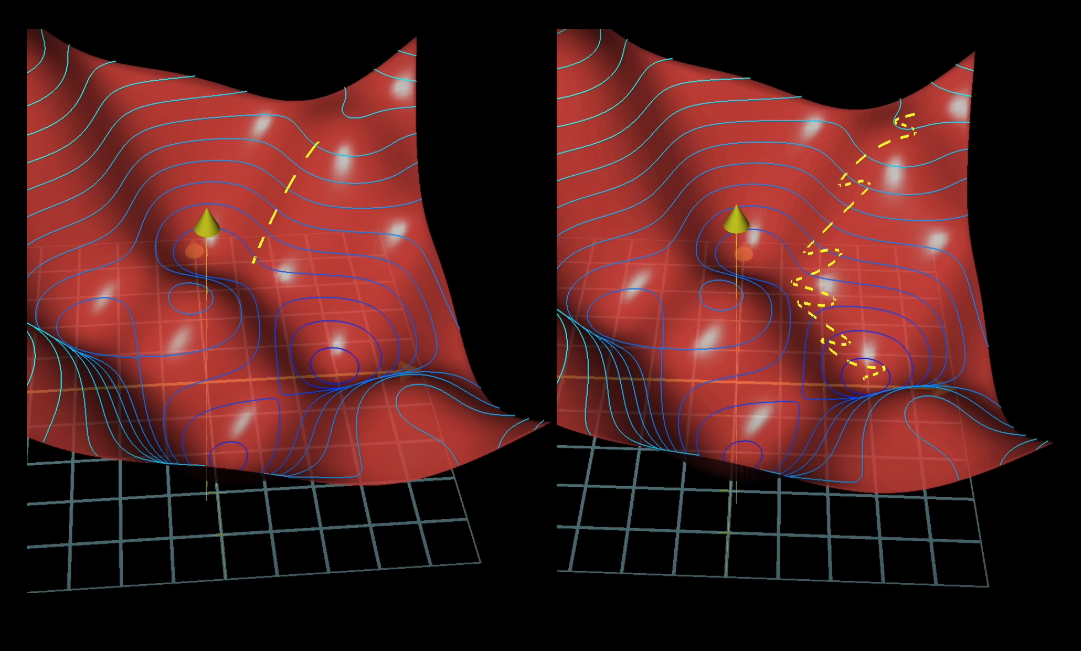
An image depiction of how the gradient descent method would look when let's a man is trying to find the way downhill from a point high up in the hills. The image on the right shows a faster variant of Gradient Descent called "Stochastic Gradient Descent" which is a method not as accurate as the original Gradient Descent, but faster than it, typically useful in deep learning. The original Gradient descent method would represent a man taking careful and calculated steps downward, which is slow, and the stochastic gradient descent method would represent a drunken man taking large abrupt steps downhill, but getting down faster.

How does this tie to here in physics? Well Gradient Descent aims to find the most steepest decrease of a particular function, just opposite to what 1. Gradient does, which finds the steepest increase or ascent.

In physics, :

• $V(x,y,z)$ is potential energy.
• The force is given by:

or :

• Why the minus sign?

  • Physical systems "want" to move toward lower potential energy.
  • Example: a ball on a hill rolls downhill (towards decreasing $V$), not uphill.
  • So the force vector points in the direction of steepest decrease of potential.

Example

Take gravitational potential near Earth:

So,

which is the familiar downward force of gravity.

Equipotential Surfaces

https://www.youtube.com/watch?v=KJSgRc9_zBs (A good video explanation but it's more related to an electric field.)

In mechanics, an equipotential surface is a three-dimensional surface where the gravitational potential energy of an object is constant, meaning no work is done in moving the object along the surface.

Just as electric field lines are always perpendicular to equipotential surfaces in electrostatics, gravitational field lines are perpendicular to equipotential surfaces in mechanics. The concept is applicable to any potential field, such as gravity, so the equipotential surfaces for a uniform gravitational field are horizontal planes.

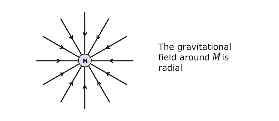
Gravitational field lines are imaginary lines used to visualize the gravitational field around a mass, with arrows indicating the direction of the attractive force and the density of the lines showing the field's strength. The lines point radially inward towards the source of the mass, and they are closer together where the field is stronger and spread out where it is weaker, such as farther from the Earth.

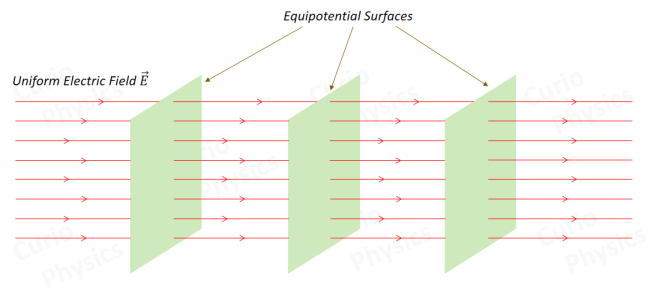
This image applies to any field, in this picture, it's an electric field shown which is perpendicular to the surface, and thus there is zero work done.

The gradient $\mathrm{\nabla }V$ is always perpendicular to equipotential surfaces, because force is normal to them.

This means that, in the above image, if we turn the field to a horizontal one, the acting force becomes a vertical one, so it's easier for us to understand:

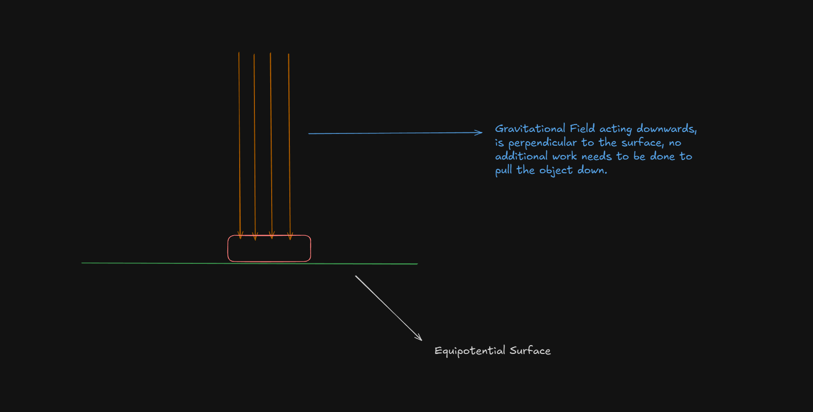
So,

Work is defined as:

(dot product of force and displacement).

On an equipotential surface, your displacement $\overrightarrow{d}$ is tangent to the surface.

The field ($F=-\mathrm{\nabla }V$) is perpendicular to the surface.

Thus,

Because the dot product vanishes, no work is needed to move along that surface.

Conservative vs Non Conservative Forces

https://www.youtube.com/watch?v=N7DAqKuSCsk

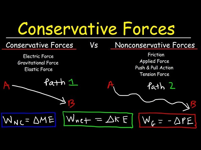
A conservative force does the same amount of work regardless of the path taken between two points, such as gravity. In contrast, a non-conservative force's work depends on the path followed, and it often dissipates mechanical energy into forms like heat or sound, with examples including friction and air resistance

1. Examples

• Conservative forces: gravity, electric force, spring force.
• Non-conservative forces: friction, air drag, applied pushes/pulls, tension in rope.

2. Path dependence

• Conservative force → path independent.
  Work only depends on start and end points.
  (e.g., gravity: lifting a ball 10 m costs the same work no matter what path you take).

• Non-conservative force → path dependent.
  Work depends on the distance traveled.
  (e.g., friction: longer path = more energy lost).

3. Example in plain words

Ball dropped from 100 m → falls to 30 m.

• At top: all potential energy (9800 J), no kinetic.
• At bottom: part converted to kinetic, part still potential.
• Total stays the same (9800 J).
• Wy? Only gravity (a conservative force) is acting.

If there were air resistance, mechanical energy would be less at the bottom → because friction/drag is non-conservative.

Conservation Laws of Energy and Momentum

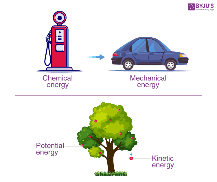
1. Law of Conservation of Energy

https://byjus.com/physics/law-of-conservation-of-energy/

• Statement:
  Energy can neither be created nor destroyed; it can only transform from one form to another, but the total energy of an isolated system remains constant.

• In mechanics:

  • Kinetic energy $K$ and potential energy $U$ may change,
  • but the total mechanical energy

- is constant if only conservative forces act.

• If non-conservative forces (like friction) are present → mechanical energy is not conserved, but total energy (including heat, sound, etc.) is still conserved.

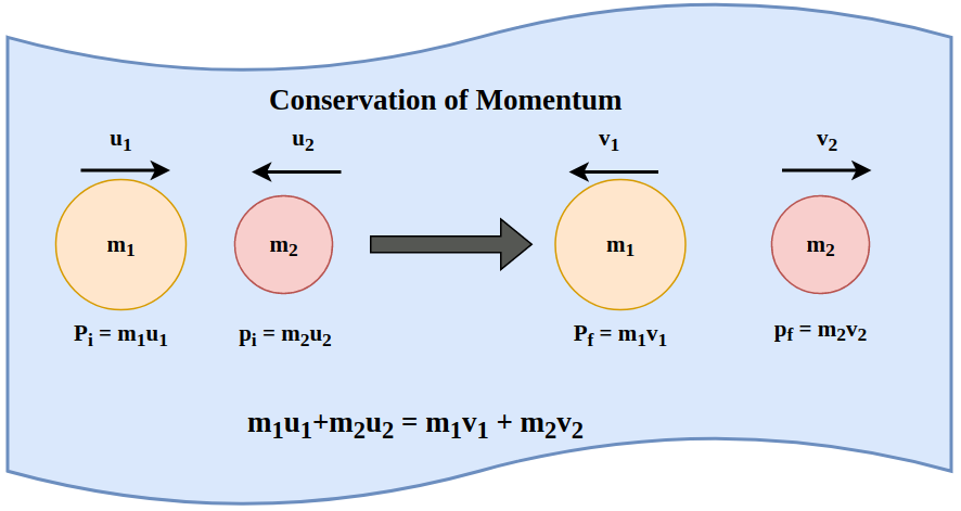
2. Law of Conservation of Linear Momentum

https://www.geeksforgeeks.org/physics/laws-of-conservation-of-momentum/

Law of Conservation of Momentum is one of the basic laws of physics which is used derived from Newton's third law of Motion. Conservation of Momentum states that the momentum of the system is always conserved, i.e. initial momentum and final momentum of the system are always conserved. We can also state that the total momentum of the system is always constant.

• Statement:
  In an isolated system (no external force), the total linear momentum remains constant:

where $\overrightarrow{p}=m\overrightarrow{v}$.

• Applies to:

  • Collisions (elastic and inelastic).
  • Explosions.

• Example: two skaters push off each other → momentum conserved in opposite directions.

Let's say the mass of the object is “m” and its velocity is “v”. Then the momentum "$\rho$" (pronounced as "rho") is given by,

So, according to the law of conservation of momentum, if two objects, having masses $m_1$ and $m_2$ and initial velocities $u_1$ and $u_2$ and final velocities $v_1$ and $v_2$ respectively, collide with each other, their initial momentum before collision and their momentum after collision is preserved.

3. Law of Conservation of Angular Momentum

The law of conservation of angular momentum states that the total angular momentum of a system remains constant when no external net torque acts on it. This means the system's rotational motion will continue unchanged in magnitude and direction.

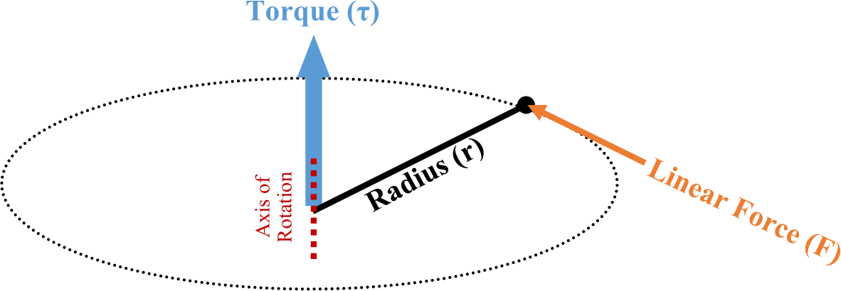
But, what is Torque?

Torque is a "twisting" or rotational force that causes an object to rotate or spin around an axis. It's the rotational equivalent of a linear force, meaning that just as force causes an object to accelerate in a straight line, torque causes an object to experience angular acceleration. You apply torque when you use a wrench to tighten a bolt or when you push on a doorknob.

The law of conservation of angular momentum is denoted by the formula:

where:

• $L$ is the angular momentum
• $I$ is the moment of inertia
• $\omega$ is the angular velocity.

Key Idea

• Energy conservation = scalar (total energy stays fixed).
• Momentum conservation = vector (both magnitude and direction matter).
• Angular momentum conservation = rotational analogue of linear momentum.

Non-inertial frame of reference

Step 1: Inertia

• Definition: The tendency of a body to resist any change in its state of motion.
• Comes directly from Newton’s First Law.
• Quantified by mass (more mass → more inertia).

Newton's first law of motion, also called the Law of Inertia, states that an object will remain at rest or in uniform motion in a straight line unless acted upon by an unbalanced net external force. In simpler terms, objects at rest stay at rest, and objects in motion continue in their state of motion (speed and direction) until a force interferes with that state.

Step 2: Frame of Reference (FoR)

• A frame of reference is a coordinate system + a clock that you use to describe motion.

• Motion is relative → velocity, acceleration, etc. are defined w.r.t a frame.

• Example:

  • Sitting in a train, the person next to you is at rest in your frame.
  • To an observer on the ground, both of you are moving with velocity of the train.

Step 3: Inertial Frame of Reference

• A frame where Newton’s laws hold.
• Either at rest or moving with constant velocity (no acceleration).
• Example: A lab fixed on Earth (ignoring rotation/curvature for basic problems).

Step 4: Non-Inertial Frame of Reference

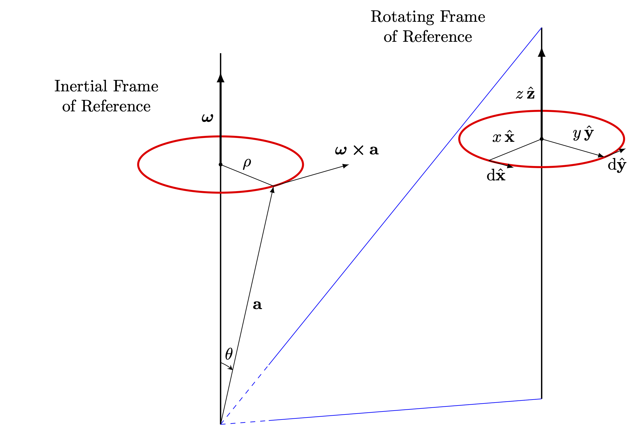
A non-inertial frame of reference is a system that is accelerating or rotating relative to an inertial frame, meaning it is not moving at a constant velocity. Diagrams of non-inertial frames often show an accelerating or rotating environment, such as a merry-go-round or an elevator, with a stationary "pseudo-force" acting on objects within it to explain their apparent acceleration. These diagrams typically compare the non-inertial frame's motion with an external, inertial frame

• A frame that is accelerating (linear or rotational).
• Newton’s laws do not directly hold here.
• To make sense of motion, you need to add fictitious/inertial forces.
  • E.g. centrifugal force, Coriolis force, pseudo-force in an accelerating car.

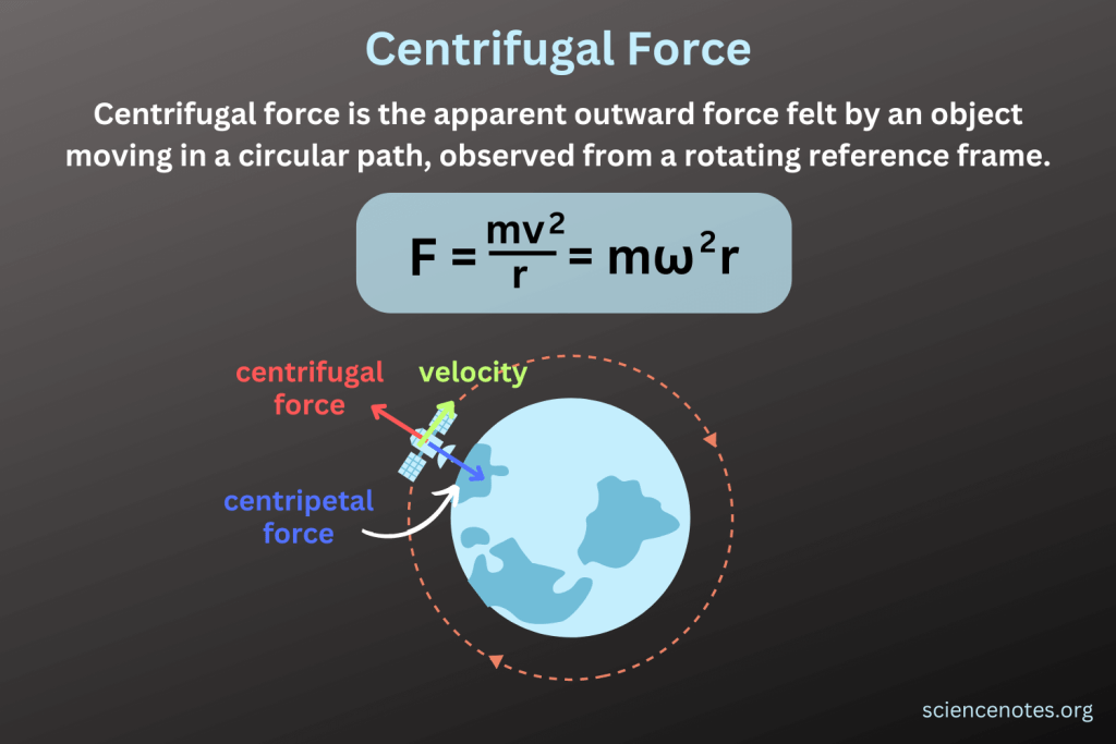
A good example for the centrifugal non-inertial frame of reference would be a satellite going around the earth, since it won't be moving at a constant velocity.

Simple Harmonic Oscillator

https://www.youtube.com/watch?v=bmGqhM-tUk4

The simple harmonic oscillator is by the simplest and most important system in physics that we going to continue to meet time and time again across different dimensions of physics, so it's imperative that we properly understand the inner workings of this system.

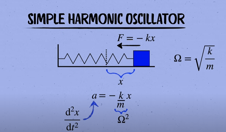
In the picture we can see the ohm symbol, in practice, all equations use $\omega$ (omega) instead.

So, we have our simple harmonic oscillator setup here where a simple square block of mass $m$ is attached to a spring whose other end is stuck to a wall.

Now, by default, the spring is at rest, or at equilibrium. The equilibrium of an object is defined by the state when all external forces and torques acting on it are balanced, resulting in zero net force and zero net torque. This balance means the object experiences no linear or angular acceleration, so it either remains at rest (static equilibrium) or moves at a constant velocity (dynamic equilibrium).

Now suppose we pull the block by a distance of $x$ . What do you think the force needed, would be, in order to get the spring back in a state of equilibrium?

That's defined by:

where $k$ is the spring constant, which denotes how "stiff" the spring is.

That minus sign is crucial — it encodes the restoring force direction (acceleration always opposite to displacement).

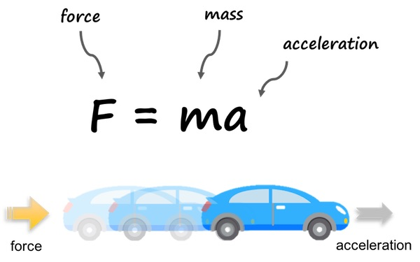
Now, from newton's second law of motion, which says:

The equation F = ma states that the net force (F) acting on an object is equal to its mass (m) multiplied by its acceleration (a). This is Newton's second law of motion which fundamentally links an object's mass and the force applied to it to the resulting acceleration it experiences.

We can say that :

or:

Now we can set $\sqrt{\frac{k}{m}}$ to a simpler constant $\omega$. This is just to simplify the equation.

So, ${\omega }^2=\frac{k}{m}$

Why Define ${\omega }^2=\frac{k}{m}$

Two reasons:

1. Simplicity — instead of always writing $\frac{k}{m}$ we use a single symbol.

2. Physical meaning — $\omega$

And the value of $\omega$ is fixed, it is determined by the stiffness of the spring $k$ and the mass of the block $m$.

Now, we can set

Why?

Acceleration is the rate of change of velocity with time.
Velocity itself is the rate of change of position with time.
So:

This is always true — not just for oscillators, but for any motion at all.

So, the equation becomes:

or :

So, the general solution of this equation is:

What are $A$ and $B$?

They are just constants determined by initial conditions.

• $A$ controls the cosine part (how much of the motion “starts as displacement”) (block being pulled, spring being stretched)

• $B$ controls the sine part (how much of the motion “starts as velocity”), block released, spring goes to and fro.

Together, they’re not “separate motions” — they combine to give the actual trajectory.

Mathematically:

• At $t=0$:

What exactly is displacement?

Displacement is a vector quantity that describes the change in position of an object from its initial location to its final location, encompassing both the shortest distance between these points and the direction of that change. It is calculated as the difference between the final position ( $x_f$ ) and the initial position ( $x_i$​ ), represented mathematically as :$s=x_f-x_i=\mathrm{\Delta }x$

• Differentiate:

At $t=0$:

Here, $C$ is the amplitude and $\varphi$ is the phase.

Again, what is the amplitude of a wave?

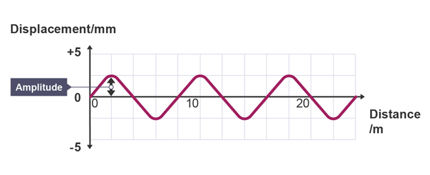
In physics, amplitude is the maximum displacement of a point on a vibrating body or a wave from its equilibrium (or resting) position. It measures the strength, intensity, or power of the wave, such as the loudness of a sound wave or the width of a water wave. For example, in a sound wave, a larger amplitude corresponds to a louder sound.

In terms of SHO, a bigger amplitude would mean a wider reach of the block (pushed by the spring), from it's initial position.

However this amplitude will get smaller with time and eventually reach zero as the spring restores itself to equilibrium, which we will study about in the next section.

And, what is the phase of a wave?

The phase of a wave represents its position or state within its cycle at a given moment in time or location. It is often expressed as an angle (in degrees or radians) and is crucial for understanding how waves interact, such as in constructive or destructive interference, where the relative phases of two waves determine if they amplify or cancel each other out.
(More on interference patterns in the next unit.)

This is just another way of writing the same thing, using trigonometric identities:

where

Graphical View

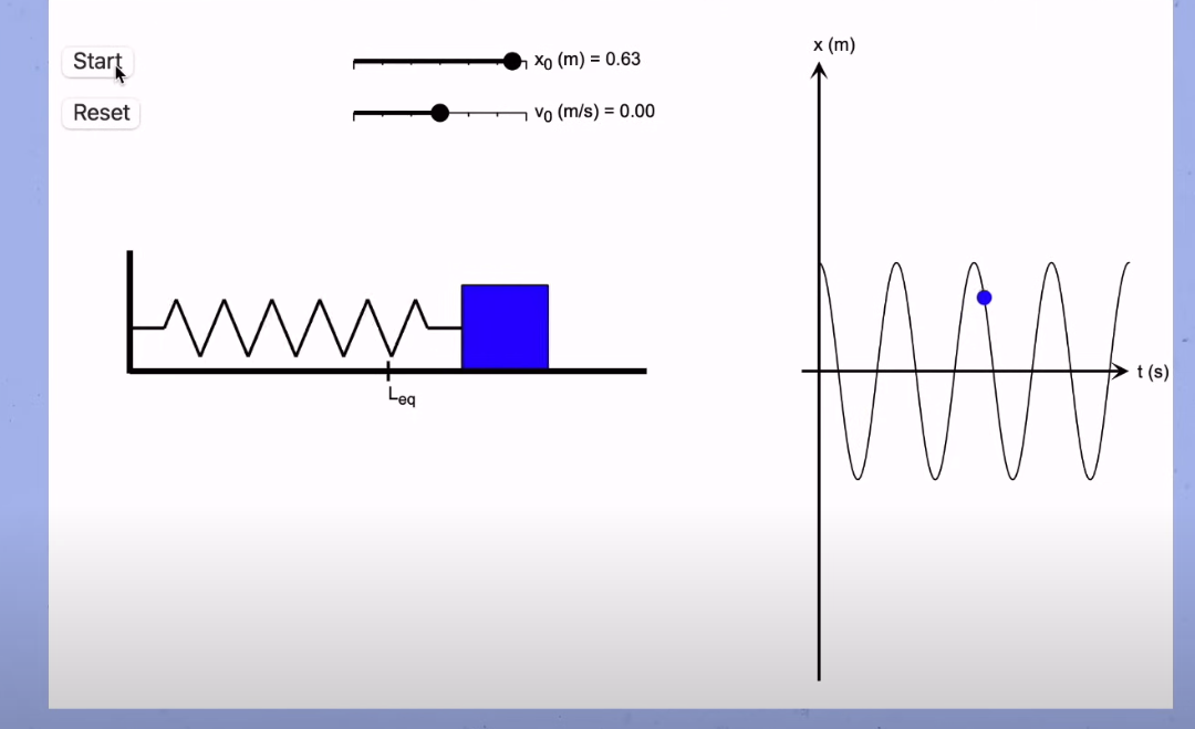
This is how the equation plotted over some $x$ and $t$ values would look.

This is a sinusoidal oscillation with amplitude and phase determined by initial conditions

Dampened harmonic motions and oscillations

Well, life's not always fair, and we don't live in an ideal world where everyone is happy and kind to each other and there are no problems, wars or any bad stuff, but that's just an ideal world. In the real dull world of ours there's all sorts of bad stuff and opposing forces acting against us. Just like it's in the case of the Simple Harmonic Oscillator. Poor thing can't even oscillate freely without some forces opposing it.

SHO (Simple Hamonic Oscillator) Recap.

So, in the ideal world, we have the equation of the Simple Harmonic Oscillator as:

where ${\omega }^2=\frac{k}{m}$, a fixed constant determined by the spring's stiffness and the mass of the block.

whose solution was:

with constant amplitude.

That’s an ideal world: no friction, no air resistance, the block would oscillate forever.

2. Real life: friction is everywhere

In reality, oscillations lose energy (to air, friction, resistance, etc.). That means the amplitude decays with time.

We model this by adding a damping force proportional to velocity:

where $b$ is the damping coefficient.

3. New equation of motion:

From newton's second law of motion:

and the restoring force of the spring:

we get:

and since in SHO, we have :

We get:

or

Adding the damping force to this:

Now this ODE is not in the perfect linear form yet, so we divide both sides by $m$.

And since ${\omega }_0=\sqrt{\frac{k}{m}}$ which is the natural undamped frequency,

We get:

Now, the damping constant, that is the rate at which the damping force increases, is given by:

Thus, :

So, the final dampened motion equation of the SHO becomes:

So damping adds a middle term proportional to velocity. That’s the mathematical fingerprint of energy loss.

So,

• No damping → simple sinusoidal solutions.
• With damping → solutions include an exponential decay factor multiplied with the sinusoid (or pure exponential if no oscillation).

Types of dampening

Now, there are three types of this dampened oscillation that the system can have, depending on the relative size of $\gamma$ and ${\omega }_0$:

(a) Underdamped case $\gamma <\omega$

• Motion is still oscillatory, but amplitude decays exponentially (in the early stages of motion of the system):

  The solution of this system can be given by:

with ${\omega }^{\prime }=\sqrt{{\omega }^2-{\gamma }^2}$

• Looks like a sinusoid with a shrinking envelope.

(b) Critically damped case $\gamma =\omega$

• System just barely avoids oscillating.
• Returns to equilibrium as fast as possible without overshoot. (almost about to stop)
• Solution is a non-oscillatory exponential.

(c) Overdamped case $\gamma >\omega$

• No oscillation (in the very last stages of stopping, to us visually, it's already stopped moving since we can't perceive that many discrete frames of motion.)
• System returns slowly to equilibrium, more sluggish than critical damping.

So, depending on the relative size of $\gamma$ and ${\omega }_0$, the system can be underdamped, critically damped or overdamped.

Physical intuition

• Underdamped: like a swing slowly coming to rest.
• Critical damping: car shock absorbers (no bounce, fastest settle).
• Overdamped: imagine moving a block through heavy honey — it takes forever to return.

Resonance (not the song)

Resonance comes in when we take our damped oscillator and drive it with an external periodic force.

From the damped SHO, we already have:

Add a driving force

Suppose an external force is applied:

Newton's law becomes:

Dividing both sides by $m$:

Now, this would get a bit more harder to solve, as not only this is a Second Order ODE, but a non-homogenous one.

What does this mean?

• The left-hand side is your oscillator with damping.
• The right-hand side is the driving force trying to shake it.

So the system’s motion will be a combination of:

1. The natural response (like before, which dies away with time due to damping).
2. The steady-state response to the driving force (which dominates long-term).

The steady state solution.

The solution to this equation looks like:

where:

• $A(\omega )=\text{amplitude(depends on driving frequency)}$
• $\varphi =\text{phase lag between force and response}$

The amplitude turns out to be:

(no need to focus on this formula too much. Just understand the gist and concepts.)

Finally, what is Resonance?

• Resonance happens when the amplitude $A(\omega )$ is maximum.
• This occurs when $\omega \approx {\omega }_0$​ (driving frequency ≈ natural frequency).
• With no damping ($\gamma =0$), amplitude theoretically goes to infinity at resonance (unphysical).
• With damping, the peak is finite, and the maximum shifts slightly to:

​
(very close to ${\omega }_0$​ if damping is weak).

Physical Intuition

• Think of a swing: if you push it in sync with its natural rhythm, the swing’s amplitude grows → resonance.
• If you push out of rhythm, you get a weaker response.
• Damping (like air resistance or friction) keeps the amplitude finite in real life.

Angular Velocity and it's vector

Angular Displacement

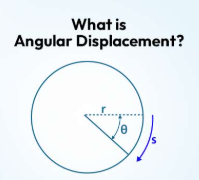
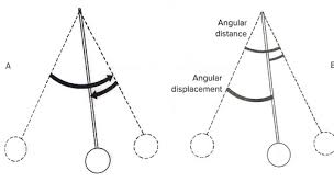
First off, let's start with angular displacement.

Angular displacement is the angle through which a body rotates around a fixed axis or center, measuring the change in its angular position over time. Unlike linear displacement, which measures straight-line distance, angular displacement quantifies how much an object has "turned" from its starting point, with units like radians or degrees. It is a vector quantity, meaning it has both magnitude (the size of the angle) and direction.

Angular Velocity

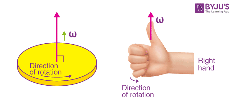
Angular velocity (symbolized by the Greek letter omega, ω) is the rate at which an object rotates, measured as the change in its angular displacement over time. It describes how fast an object is turning and in what direction. The SI unit for angular velocity is radians per second (rad/s), though other units like degrees per second and revolutions per minute (RPM) are also used

Angular velocity is a vector, meaning it has both magnitude (speed of rotation) and direction.

The direction is often determined by the right-hand rule. If you curl your fingers around the axis of rotation in the direction of the object's spin, your thumb points in the direction of the angular velocity vector. It's also known as Fleming's right-hand rule.

Formula of Angular Velocity

The angular velocity $\omega$, is given by:

where:

• $\omega =\text{the angular velocity}$
• $\mathrm{\Delta }\theta =\text{change in angular rotation / angular displacement}$
• $\mathrm{\Delta }t=\text{change in time}$

Relation of Angular Velocity to Linear Velocity.

For a point at position $\overrightarrow{r}$ with angular velocity $\overrightarrow{\omega }$ ,

The linear velocity vector, $\overrightarrow{v}$, is given by:

This connects angular velocity with the actual linear speed of a particle.

Angular Acceleration

Just like linear velocity changes give acceleration, changes in angular velocity give:

6. Examples

• A wheel spinning at $10\text{rad/s}$: its angular velocity vector points along the axle.
• Earth’s rotation: $\omega \approx 7.27\times {10}^{-5}\text{rad/s}$, vector pointing along Earth’s axis (north pole direction).

Moment of Inertia

Moment of inertia is a measure of an object's resistance to changes in its rotational motion, analogous to how mass resists changes in linear motion. It depends on the object's mass, how that mass is distributed relative to the axis of rotation, and the specific axis chosen. Greater mass or mass located further from the axis of rotation results in a higher moment of inertia, making it harder to start or stop the object's rotation.

Formula

The formula of the moment of inertia is given by:

where:

• $I$ is the inertia
• $L$ is the angular momentum
• $\omega$ is the angular velocity